Implement Incremental Learning for Regression Using Flexible Workflow
This example shows how to use the flexible workflow to implement incremental learning for linear regression with prequential evaluation. A traditionally trained model initializes the incremental model. Specifically, this example does the following:
Train a linear regression model on a subset of data.
Convert the traditionally trained model to an incremental learning model for linear regression.
Simulate a data stream using a for loop, which feeds small chunks of observations to the incremental learning algorithm.
For each chunk, use
updateMetricsto measure the model performance given the incoming data, and then usefitto fit the model to that data.
Load and Preprocess Data
Load the 2015 NYC housing data set, and shuffle the data. For more details on the data, see NYC Open Data.
load NYCHousing2015
rng(1) % For reproducibility
n = size(NYCHousing2015,1);
idxshuff = randsample(n,n);
NYCHousing2015 = NYCHousing2015(idxshuff,:);
Suppose that the data collected from Manhattan (BOROUGH = 1) was collected using a new method that doubles its quality. Create a weight variable that attributes 2 to observations collected from Manhattan, and 1 to all other observations.
NYCHousing2015.W = ones(n,1) + (NYCHousing2015.BOROUGH == 1);
Extract the response variable SALEPRICE from the table. For numerical stability, scale SALEPRICE by 1e6.
Y = NYCHousing2015.SALEPRICE/1e6;
NYCHousing2015.SALEPRICE = [];
Create dummy variable matrices from the categorical predictors.
catvars = ["BOROUGH" "BUILDINGCLASSCATEGORY" "NEIGHBORHOOD"];
dumvarstbl = varfun(@(x)dummyvar(categorical(x)),NYCHousing2015,...
    'InputVariables',catvars);
dumvarmat = table2array(dumvarstbl);
NYCHousing2015(:,catvars) = [];
Treat all other numeric variables in the table as linear predictors of sales price. Concatenate the matrix of dummy variables to the rest of the predictor data. Transpose the data.
idxnum = varfun(@isnumeric,NYCHousing2015,'OutputFormat','uniform');
X = [dumvarmat NYCHousing2015{:,idxnum}]';
Train Linear Regression Model
Fit a linear regression model to a random sample of half the data. Specify that observations are oriented along the columns of the data.
idxtt = randsample([true false],n,true);
TTMdl = fitrlinear(X(:,idxtt),Y(idxtt),'ObservationsIn','columns')
TTMdl =
  RegressionLinear
         ResponseName: 'Y'
    ResponseTransform: 'none'
                 Beta: [313×1 double]
                 Bias: 0.1889
               Lambda: 2.1977e-05
              Learner: 'svm'


  Properties, Methods
TTMdl is a RegressionLinear model object representing a traditionally trained linear regression model.
Convert Trained Model
Convert the traditionally trained linear regression model to a linear regression model for incremental learning.
IncrementalMdl = incrementalLearner(TTMdl)
IncrementalMdl =
  incrementalRegressionLinear

               IsWarm: 1
              Metrics: [1×2 table]
    ResponseTransform: 'none'
                 Beta: [313×1 double]
                 Bias: 0.1889
              Learner: 'svm'


  Properties, Methods
Implement Incremental Learning
Use the flexible workflow to update model performance metrics and fit the incremental model to the training data by calling the updateMetrics and fit functions separately. Simulate a data stream by processing 500 observations at a time. At each iteration:
Call
updateMetricsto update the cumulative and window epsilon insensitive loss of the model given the incoming chunk of observations. Overwrite the previous incremental model to update the losses in theMetricsproperty. Note that the function does not fit the model to the chunk of data—the chunk is "new" data for the model. Specify that observations are oriented along the columns of the data.Call
fitto fit the model to the incoming chunk of observations. Overwrite the previous incremental model to update the model parameters. Specify that observations are oriented along the columns of the data.Store the losses and last estimated coefficient .
% Preallocation
numObsPerChunk = 500;
nchunk = floor(n/numObsPerChunk);
ei = array2table(zeros(nchunk,2),'VariableNames',["Cumulative" "Window"]);
beta313 = zeros(nchunk,1);

% Incremental fitting
for j = 1:nchunk
    ibegin = min(n,numObsPerChunk*(j-1) + 1);
    iend   = min(n,numObsPerChunk*j);
    idx = ibegin:iend;
    IncrementalMdl = updateMetrics(IncrementalMdl,X(:,idx),Y(idx),'ObservationsIn','columns');
    ei{j,:} = IncrementalMdl.Metrics{"EpsilonInsensitiveLoss",:};
    IncrementalMdl = fit(IncrementalMdl,X(:,idx),Y(idx),'ObservationsIn','columns');
    beta313(j) = IncrementalMdl.Beta(end);
end
IncrementalMdl is an incrementalRegressionLinear model object trained on all the data in the stream.
Alternatively, you can use updateMetricsAndFit to update performance metrics of the model given a new chunk of data, and then fit the model to the data.
Inspect Model Evolution
Plot a trace plot of the performance metrics and estimated coefficient .
t = tiledlayout(2,1);
nexttile
h = plot(ei.Variables);
xlim([0 nchunk])
ylabel('Epsilon Insensitive Loss')
legend(h,ei.Properties.VariableNames)
nexttile
plot(beta313)
ylabel('\beta_{313}')
xlim([0 nchunk])
xlabel(t,'Iteration')
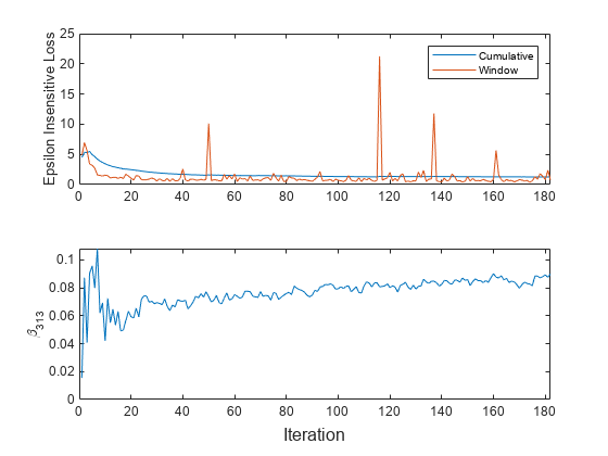
The cumulative loss gradually changes with each iteration (chunk of 500 observations), whereas the window loss jumps. Because the metrics window is 200 by default, updateMetrics measures the performance based on the latest 200 observations in each 500 observation chunk.
changes abruptly at first and then just slightly as fit processes chunks of observations.