Fit Kernel Distribution Using ksdensity

This example shows how to generate a kernel probability density estimate from sample data using the ksdensity function.

Step 1. Load sample data.

Load the sample data.

load carsmall;

This data contains miles per gallon (MPG) measurements for different makes and models of cars, grouped by country of origin (Origin), model year (Year), and other vehicle characteristics.

Step 2. Generate a kernel probability density estimate.

Use ksdensity to generate a kernel probability density estimate for the miles per gallon (MPG) data.

[f,xi] = ksdensity(MPG);

By default, ksdensity uses a normal kernel smoothing function and chooses an optimal bandwidth for estimating normal densities, unless you specify otherwise.

Step 3. Plot the kernel probability density estimate.

Plot the kernel probability density estimate to visualize the MPG distribution.

plot(xi,f,'LineWidth',2)
title('Miles per Gallon')
xlabel('MPG')

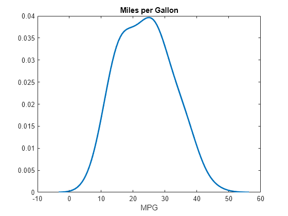
The plot shows the pdf of the kernel distribution fit to the MPG data across all makes of cars. The distribution is smooth and fairly symmetrical, although it is slightly skewed with a heavier right tail.