Bayesian Linear Regression Using Hamiltonian Monte Carlo
This example shows how to perform Bayesian inference on a linear regression model using a Hamiltonian Monte Carlo (HMC) sampler.
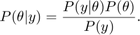
In Bayesian parameter inference, the goal is to analyze statistical models with the incorporation of prior knowledge of model parameters. The posterior distribution of the free parameters  combines the likelihood function
  with the prior distribution
  , using Bayes' theorem:
Usually, the best way to summarize the posterior distribution is to obtain samples from that distribution using Monte Carlo methods. Using these samples, you can estimate marginal posterior distributions and derived statistics such as the posterior mean, median, and standard deviation. HMC is a gradient-based Markov Chain Monte Carlo sampler that can be more efficient than standard samplers, especially for medium-dimensional and high-dimensional problems.
Linear Regression Model
Analyze a linear regression model with the intercept  , the linear coefficients
  (a column vector), and the noise variance
  of the data distribution as free parameters. Assume that each data point has an independent Gaussian distribution:

Model the mean  of the Gaussian distribution as a function of the predictors
  and model parameters as

In a Bayesian analysis, you also must assign prior distributions to all free parameters. Assign independent Gaussian priors on the intercept and linear coefficients:
 ,
,
 .
.
To use HMC, all sampling variables must be unconstrained, meaning that the posterior density and its gradient must be well-defined for all real parameter values. If you have a parameter that is constrained to an interval, then you must transform this parameter into an unbounded one. To conserve probability, you must multiply the prior distribution by the corresponding Jacobian factor. Also, take this factor into account when calculating the gradient of the posterior.
The noise variance is a (squared) scale parameter that can only be positive. It then can be easier and more natural to consider its logarithm as the free parameter, which is unbounded. Assign a normal prior to the logarithm of the noise variance:
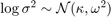 .
.
Write the logarithm of the posterior density of the free parameters 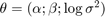 as
as

Ignore the constant term and call the sum of the last two terms  . To use HMC, create a function handle that evaluates and its gradient
  for any value of . The functions used to calculate are located at the end of the script.
Create Data Set
Define true parameter values for the intercept, the linear coefficients Beta, and the noise standard deviation. Knowing the true parameter values makes it possible to compare with the output of the HMC sampler. Only the first predictor affects the response.
NumPredictors = 2;

trueIntercept = 2;
trueBeta = [3;0];
trueNoiseSigma = 1;
Use these parameter values to create a normally distributed sample data set at random values of the two predictors.
NumData = 100;
rng('default') %For reproducibility
X = rand(NumData,NumPredictors);
mu = X*trueBeta + trueIntercept;
y = normrnd(mu,trueNoiseSigma);
Define Posterior Probability Density
Choose the means and standard deviations of the Gaussian priors.
InterceptPriorMean = 0;
InterceptPriorSigma = 10;
BetaPriorMean = 0;
BetaPriorSigma = 10;
LogNoiseVarianceMean = 0;
LogNoiseVarianceSigma = 2;
Save a function logPosterior on the MATLAB® path that returns the logarithm of the product of the prior and likelihood, and the gradient of this logarithm. The logPosterior function is defined at the end of this example. Then, call the function with arguments to define the logpdf input argument to the hmcSampler function.
logpdf = @(Parameters)logPosterior(Parameters,X,y, ...
    InterceptPriorMean,InterceptPriorSigma, ...
    BetaPriorMean,BetaPriorSigma, ...
    LogNoiseVarianceMean,LogNoiseVarianceSigma);
Create HMC Sampler
Define the initial point to start sampling from, and then call the hmcSampler function to create the Hamiltonian sampler as a HamiltonianSampler object. Display the sampler properties.
Intercept = randn;
Beta = randn(NumPredictors,1);
LogNoiseVariance = randn;
startpoint = [Intercept;Beta;LogNoiseVariance];
smp = hmcSampler(logpdf,startpoint,'NumSteps',50);
smp
smp =

  HamiltonianSampler with properties:

                  StepSize: 0.1000
                  NumSteps: 50
                MassVector: [4×1 double]
              JitterMethod: 'jitter-both'
      StepSizeTuningMethod: 'dual-averaging'
    MassVectorTuningMethod: 'iterative-sampling'
                    LogPDF: [function_handle]
             VariableNames: {4×1 cell}
                StartPoint: [4×1 double]
Estimate MAP Point
Estimate the MAP (maximum-a-posteriori) point of the posterior density. You can start sampling from any point, but it is often more efficient to estimate the MAP point, and then use it as a starting point for tuning the sampler and drawing samples. Estimate and display the MAP point. You can show more information during optimization by setting the 'VerbosityLevel' value to 1.
[MAPpars,fitInfo] = estimateMAP(smp,'VerbosityLevel',0);
MAPIntercept = MAPpars(1)
MAPBeta = MAPpars(2:end-1)
MAPLogNoiseVariance = MAPpars(end)
MAPIntercept =

    2.3857


MAPBeta =

    2.5495
   -0.4508


MAPLogNoiseVariance =

   -0.1007
To check that the optimization has converged to a local optimum, plot the fitInfo.Objective field. This field contains the values of the negative log density at each iteration of the function optimization. The final values are all similar, so the optimization has converged.
plot(fitInfo.Iteration,fitInfo.Objective,'ro-');
xlabel('Iteration');
ylabel('Negative log density');

Tune Sampler
It is important to select good values for the sampler parameters to get efficient sampling. The best way to find good values is to automatically tune the MassVector, StepSize, and NumSteps parameters using the tuneSampler method. Use the method to:
1. Tune the MassVector of the sampler.
2. Tune StepSize and NumSteps for a fixed simulation length to achieve a certain acceptance ratio. The default target acceptance ratio of 0.65 is good in most cases.
Start tuning at the estimated MAP point for more efficient tuning.
[smp,tuneinfo] = tuneSampler(smp,'Start',MAPpars);
Plot the evolution of the step size during tuning to ensure that the step size tuning has converged. Display the achieved acceptance ratio.
figure;
plot(tuneinfo.StepSizeTuningInfo.StepSizeProfile);
xlabel('Iteration');
ylabel('Step size');

accratio = tuneinfo.StepSizeTuningInfo.AcceptanceRatio
accratio =

    0.6100

Draw Samples
Draw samples from the posterior density, using a few independent chains. Choose different initial points for the chains, randomly distributed around the estimated MAP point. Specify the number of burn-in samples to discard from the beginning of the Markov chain and the number of samples to generate after the burn-in.
Set the 'VerbosityLevel' value to print details during sampling for the first chain.
NumChains = 4;
chains = cell(NumChains,1);
Burnin = 500;
NumSamples = 1000;
for c = 1:NumChains
    if (c == 1)
        level = 1;
    else
        level = 0;
    end
    chains{c} = drawSamples(smp,'Start',MAPpars + randn(size(MAPpars)), ...
        'Burnin',Burnin,'NumSamples',NumSamples, ...
        'VerbosityLevel',level,'NumPrint',300);
end
|==================================================================================|
|   ITER   |    LOG PDF    |  STEP SIZE  |  NUM STEPS  |  ACC RATIO  |  DIVERGENT  |
|==================================================================================|
|      300 | -1.483297e+02 |   2.685e-01 |          11 |   9.400e-01 |           0 |
|      600 | -1.494954e+02 |   2.256e-02 |           3 |   9.333e-01 |           0 |
|      900 | -1.506495e+02 |   2.302e-01 |           5 |   9.367e-01 |           0 |
|     1200 | -1.493671e+02 |   1.196e-01 |          15 |   9.333e-01 |           0 |
|     1500 | -1.497867e+02 |   2.685e-01 |          11 |   9.347e-01 |           0 |
Examine Convergence Diagnostics
Use the diagnostics method to compute standard MCMC diagnostics. For each sampling parameter, the method uses all the chains to compute these statistics:
Posterior mean estimate (
Mean)Estimate of the Monte Carlo standard error (
MCSE), which is the standard deviation of the posterior mean estimateEstimate of the posterior standard deviation (
SD)Estimates of the 5th and 95th quantiles of the marginal posterior distribution (
Q5andQ95)Effective sample size for the posterior mean estimate (
ESS)Gelman-Rubin convergence statistic (
RHat). As a rule of thumb, values ofRHatless than1.1are interpreted as a sign that the chain has converged to the desired distribution. IfRHatfor any variable is larger than1.1, then try drawing more samples using thedrawSamplesmethod.
Display the diagnostics table and the true values of the sampling parameters defined in the beginning of the example. Since the prior distribution is noninformative for this data set, the true values are between (or near) the 5th and 95th quantiles.
diags = diagnostics(smp,chains)
truePars = [trueIntercept;trueBeta;log(trueNoiseSigma^2)]
diags =

  4×8 table

     Name       Mean         MCSE         SD          Q5         Q95       ESS       RHat
    ______    _________    _________    _______    ________    _______    ______    ______

    {'x1'}       2.3773    0.0052946    0.27713      1.9058     2.8338    2739.7    1.0003
    {'x2'}        2.555    0.0061179    0.32956      2.0209     3.0982    2901.8         1
    {'x3'}     -0.44378    0.0063994    0.34008     -1.0302    0.10801    2824.2         1
    {'x4'}    -0.059179    0.0029785    0.14177    -0.28079    0.18477    2265.6    1.0008


truePars =

     2
     3
     0
     0
Visualize Samples
Investigate issues such as convergence and mixing to determine whether the drawn samples represent a reasonable set of random realizations from the target distribution. To examine the output, plot the trace plots of the samples using the first chain.
The drawSamples method discards burn-in samples from the beginning of the Markov chain to reduce the effect of the sampling starting point. Furthermore, the trace plots look like high-frequency noise, without any visible long-range correlation between the samples. This behavior indicates that the chain is mixed well.
figure;
subplot(2,2,1);
plot(chains{1}(:,1));
title(sprintf('Intercept, Chain 1'));
for p = 2:1+NumPredictors
    subplot(2,2,p);
    plot(chains{1}(:,p));
    title(sprintf('Beta(%d), Chain 1',p-1));
end
subplot(2,2,4);
plot(chains{1}(:,end));
title(sprintf('LogNoiseVariance, Chain 1'));

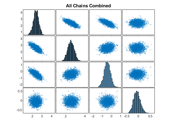
Combine the chains into one matrix and create scatter plots and histograms to visualize the 1-D and 2-D marginal posterior distributions.
concatenatedSamples = vertcat(chains{:});
figure;
plotmatrix(concatenatedSamples);
title('All Chains Combined');
Functions for Computing Posterior Distribution
The logPosterior function returns the logarithm of the product of a normal likelihood and a normal prior for the linear model. The input argument Parameter has the format [Intercept;Beta;LogNoiseVariance]. X and Y contain the values of the predictors and response, respectively.
The normalPrior function returns the logarithm of the multivariate normal probability density with means Mu and standard deviations Sigma, specified as scalars or columns vectors the same length as P. The second output argument is the corresponding gradient.
function [logpdf, gradlogpdf] = logPosterior(Parameters,X,Y, ...
    InterceptPriorMean,InterceptPriorSigma, ...
    BetaPriorMean,BetaPriorSigma, ...
    LogNoiseVarianceMean,LogNoiseVarianceSigma)


% Unpack the parameter vector
Intercept        = Parameters(1);
Beta             = Parameters(2:end-1);
LogNoiseVariance = Parameters(end);
% Compute the log likelihood and its gradient
Sigma                   = sqrt(exp(LogNoiseVariance));
Mu                      = X*Beta + Intercept;
Z                       = (Y - Mu)/Sigma;
loglik                  = sum(-log(Sigma) - .5*log(2*pi) - .5*Z.^2);
gradIntercept1          = sum(Z/Sigma);
gradBeta1               = X'*Z/Sigma;
gradLogNoiseVariance1	= sum(-.5 + .5*(Z.^2));
% Compute log priors and gradients
[LPIntercept, gradIntercept2]           = normalPrior(Intercept,InterceptPriorMean,InterceptPriorSigma);
[LPBeta, gradBeta2]                     = normalPrior(Beta,BetaPriorMean,BetaPriorSigma);
[LPLogNoiseVar, gradLogNoiseVariance2]  = normalPrior(LogNoiseVariance,LogNoiseVarianceMean,LogNoiseVarianceSigma);
logprior                                = LPIntercept + LPBeta + LPLogNoiseVar;
% Return the log posterior and its gradient
logpdf               = loglik + logprior;
gradIntercept        = gradIntercept1 + gradIntercept2;
gradBeta             = gradBeta1 + gradBeta2;
gradLogNoiseVariance = gradLogNoiseVariance1 + gradLogNoiseVariance2;
gradlogpdf           = [gradIntercept;gradBeta;gradLogNoiseVariance];
end

function [logpdf,gradlogpdf] = normalPrior(P,Mu,Sigma)
Z          = (P - Mu)./Sigma;
logpdf     = sum(-log(Sigma) - .5*log(2*pi) - .5*(Z.^2));
gradlogpdf = -Z./Sigma;
end