Execute and Unit Test Stateflow Chart Objects
A standalone Stateflow® chart is a MATLAB® class that defines the behavior of a finite state machine. Standalone charts implement classic chart semantics with MATLAB as the action language. You can program the chart by using the full functionality of MATLAB, including those functions that are restricted for code generation in Simulink®. For more information, see Create Stateflow Charts for Execution as MATLAB Objects.
Example of a Standalone Stateflow Chart
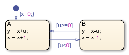
The file sf_chart.sfx contains the standalone Stateflow chart sf_chart. The chart has local data u, x, and y.
This example shows how to execute this chart from the Stateflow Editor and in the MATLAB Command Window.
Execute a Standalone Chart from the Stateflow Editor
To unit test and debug a standalone chart, you can execute the chart directly from the Stateflow Editor. During execution, you enter data values and broadcast events from the user interface.
Open the chart in the Stateflow Editor:
edit sf_chart.sfxIn the Symbols pane, enter a value of
u= 1 and click Run . The chart executes its default
transition and:
. The chart executes its default
transition and:Initializes
xto the value of 0.Makes state
Athe active state.Assigns
yto the value of 1.Increases the value of
xto 1.
The chart animation highlights the active state
A. The Symbols pane displays the valuesu= 1,x= 1, andy= 1. The chart maintains its current state and local data until the next execution command.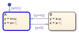
Click Step
 . Because the value of
 udoes not satisfy the condition[u<0]to transition out of stateA, this state remains active and the values ofxandyincrease to 2. The Symbols pane now displays the valuesu= 1,x= 2, andy= 2.In the Symbols pane, enter a value of
u= −1 and click Step. The negative data value triggers the transition to
state B. The Symbols pane displays the valuesu= −1,x= 1, andy= 3.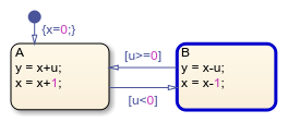
You can modify the value of any chart data in the Symbols pane. For example, enter a value of
x= 3. The chart will use this data value in the next time execution step.Enter a value of
u= 2 and click Step. The chart transitions back to state
A. The Symbols pane displays the valuesu= 2,x= 4, andy= 5.To stop the chart animation, click Stop
 .
.
To interrupt the execution and step through each action in the chart, add breakpoints before you execute the chart. For more information, see Debug a Standalone Stateflow Chart.
Execute a Standalone Chart in MATLAB
You can execute a standalone chart in MATLAB without opening the Stateflow Editor. If the chart is open, then the editor highlights active states and transitions through chart animation.
Open the chart in the Stateflow Editor. In the MATLAB Command Window, enter:
edit sf_chart.sfxCreate the Stateflow chart object by using the name of the
sfxfile for the standalone chart as a function. Specify the initial value for the datauas a name-value pair.s = sf_chart(u=1)
This command creates the chart objectStateflow Chart Execution Function y = step(s) Local Data u : 1 x : 1 y : 1 Active States: {'A'}s, executes the default transition, and initializes the values ofxandy. The Stateflow Editor animates the chart and highlights the active stateA.To execute the chart, call the
stepfunction. For example, suppose that you call thestepfunction with a value ofu= 1:step(s,u=1)
disp(s)
Because the value ofStateflow Chart Execution Function y = step(s) Local Data u : 1 x : 2 y : 2 Active States: {'A'}udoes not satisfy the condition[u<0]to transition out of stateA, this state remains active and the values ofxandyincrease to 2.Execute the chart again, this time with a value of
u= −1:step(s,u=-1)
disp(s)
The negative data value triggers the transition to stateStateflow Chart Execution Function y = step(s) Local Data u : -1 x : 1 y : 3 Active States: {'B'}B. The value ofxdecreases to 1 and the value ofyincreases to 3.To access the value of any chart data, use dot notation. For example, you can assign a value of 3 to the local data
xby entering:s.x = 3
The standalone chart will use this data value in the next time execution step.Stateflow Chart Execution Function y = step(s) Local Data u : -1 x : 3 y : 3 Active States: {'B'}Execute the chart with a value of
u= 2:step(s,u=2)
disp(s)
The chart transitions back to stateStateflow Chart Execution Function y = step(s) Local Data u : 2 x : 4 y : 5 Active States: {'A'}Aand modifies the values ofxandy.To stop the chart animation, delete the Stateflow chart object
s:delete(s)
Execute Multiple Chart Objects
You can execute multiple chart objects defined by the same standalone chart. Concurrent chart objects maintain their internal state independently, but remain associated to the same chart in the editor. The chart animation reflects the state of the chart object most recently executed. Executing multiple chart objects while the Stateflow Editor is open can produce confusing results and is not recommended.