Parameterize Magnetic Core Block Using B-H Curve Data
This example shows how to parameterize a Magnetic Core block using B-H curve data. This block represents a magnetic core with magnetic hysteresis implementing a Jiles-Atherton model.
Open Model
Open the parameterizeIronCoreWithBHCurve model.
myModel = "parameterizeIronCoreWithBHCurve";
open_system(myModel)
In this example, you model a core that an Electromagnetic Converter block magnetizes. To parameterize the model with B-H curve data, you set the Parameterization option parameter of the Magnetic Core block to Saturated BH Curve. The Magnetic flux density, B(H) and Magnetic field intensity, H parameters represent the ascendent or descendent half of the B-H curve.
Import B-H Curve
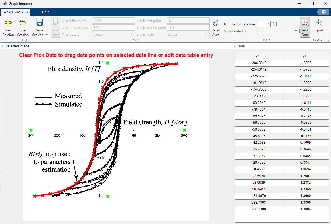
Select a saturated B-H curve chart and use the graphImporter app to capture either the ascending or descending curve.
Open the Graph Data Extractor app and open the session parameterizeIronCoreWithBHCurveGraphImporterSession.mat.

Click Export and save the data with the name BHCurve.mat. To assign the data to the corresponding variable in the workspace, load the MAT file.
load parameterizeIronCoreWithBHCurve.mat
Hdescendent = tableData(:,1);
Bdescendent = tableData(:,2);
Alternatively, you can follow the steps in the Graph Data Extractor examples to extract the B-H curve data from parameterizeIronCoreWithBHCurveFig.png.
Use the default values for the Effective length and Effective cross-sectional area parameters of the Magnetic Core block. If these values are incompatible with your B-H curves, you can change these values later.
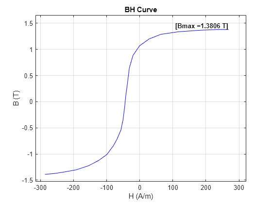
You can estimate an appropriate value for the Magnetic flux density at saturation point using the curve you imported earlier. Plot the data to visualize the saturation point.
parameterizeIronCoreWithBHCurvePlotImportedCurve

The maximum value of the imported curve is 2.2 T. However, the curve has not yet reached a plateau, so the actual flux density at the saturation point is higher than this value. Set the Magnetic flux density at saturation point parameter to 7.5% above the maximum value.
Bsaturation = max(Bdescendent)*1.075;
To define the input signal to the Controlled Voltage Source block, choose a sensible value for the Frequency (rad/sec) parameter of the Sine Wave block. In this example, you do not model eddy current losses, so choose any suitable value.
f = 1e3;
Choose a value for the Amplitude parameter of the Sine Wave block such that the electrical network provides sufficient voltage to saturate the B-H curve, but does not saturate it excessively. The resistance is equal to 1 ohm, so the voltage is equal to the current. From the previous figure, you can estimate that the saturation value for the magnetic field intensity is around 500 A/m. Set the Amplitude parameter of the Sine Wave block to 500 multiplied by the value of the Effective length parameter of the Magnetic Core block.
mmfSat = 500*meanMagneticLength;
Plot Simulation Results
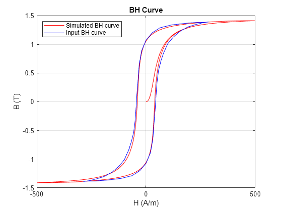
Simulate the model and plot the simulated and the input B-H curves.
parameterizeIronCoreWithBHCurvePlotCurve

The simulated curve overlaps well with the input data.
Investigate Sensitivity to Magnetic Flux Density at Saturation Point
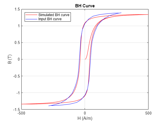
To see the importance of parameterizing your model using an appropriate saturation point, set the Magnetic flux density at saturation point parameter to the maximum value from the input data. Plot the B-H curve.
Bsaturation = max(Bdescendent);
parameterizeIronCoreWithBHCurvePlotCurve

The simulated B-H curve no longer overlaps with the input data at high flux density magnitudes.
Reset the Magnetic flux density at saturation point parameter to 7.5% above the maximum value from the input data.
Bsaturation = max(Bdescendent)*1.075;