Surrogate Optimization Using the Response Optimizer App

This example shows how to use surrogate optimization in Simulink® Design Optimization™ to optimize the design of a hydraulic cylinder, using the Response Optimizer app.

This example requires Parallel Computing Toolbox™ software.

Surrogate Optimization

Solving optimization problems involves using different values of the design variables and evaluating the objective function multiple times, especially if the objective function is sufficiently nonsmooth such that a derivative-based solver is not suitable. In such cases, you might need to use a derivative-free solver such as patternsearch, but these solvers tend to require running the objective function many more times. Using such a solver can be time consuming if the objective function is computationally expensive to evaluate. One way to overcome this problem is surrogate optimization. This approach creates a surrogate of the expensive objective function. The surrogate can be evaluated quickly and gives results very similar to the original objective function. Surrogate optimization also tries many starting points, which helps find a global optimum, rather than converging on a solution that, while locally optimal, might not be the global optimum.

Hydraulic Cylinder Model

This example shows how to use surrogate optimization to optimize the response of a hydraulic cylinder. Open the model.

open_system('sdoHydraulicCylinder')

The hydraulic cylinder model is based on the Simulink model sldemo_hydcyl. The model includes:

• Pump and Cylinder Assembly subsystems. For more information on the subsystems, see Single Hydraulic Cylinder Simulation.

• A step change applied to the cylinder control valve orifice area that causes the cylinder piston position to change.

Set Up Optimization Problem

You will use the Response Optimizer app to solve an optimization problem for this model. In the model, use the Apps tab to launch Response Optimizer. In the app, navigate to Open Session, select Open from file, and open the file sdoHydraulicCylinder_sdosession.mat. This configures the app with the optimization problem already set up.

In the optimization problem, two design variables in the model are being optimized. These are the cylinder cross-sectional area Ac and the piston spring constant K. There are two design requirements to be satisfied:

• The pressure stays under 1,750,000 N/m. This requirement is named MaxPressure in the data browser of the app. It is a requirement on the Pressures signal in the model, which is an output of the Cylinder Assembly block.

• The piston position step response satisfies a rise time of 0.04 seconds and a settling time of 0.05 seconds. This requirement is named PistonResponse in the data browser. It is a requirement on the PistonPosition signal in the model, which is another output of the Cylinder Assembly block.

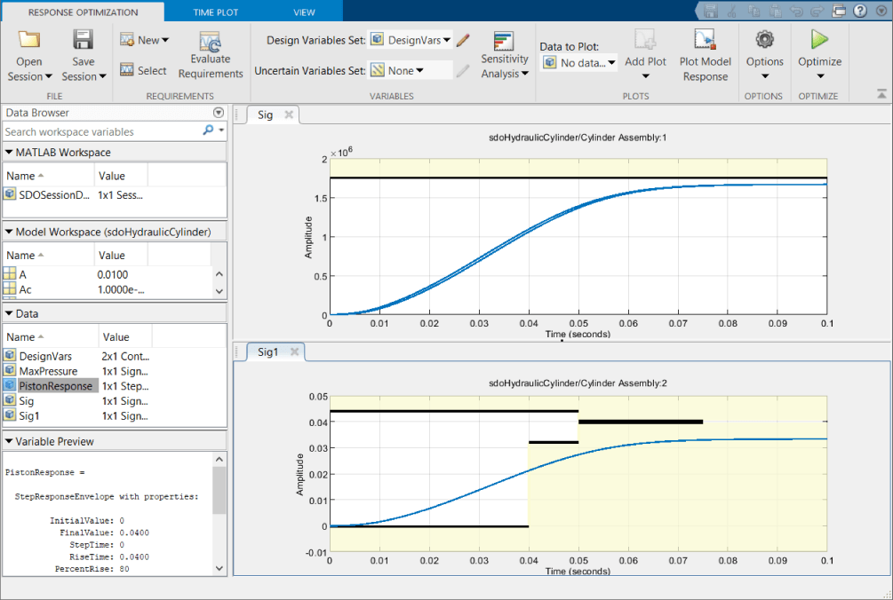
These requirements constitute the objective function which you want the optimization to satisfy. Click Plot Model Response in the toolstrip of the app. With the current values of the design variables, the pressure does satisfy the bound requirement, but the piston position curve goes into the yellow area in the plot, violating the step response requirement. To satisfy both requirements, the optimization algorithm will run the model many times with different values for the design variables, check whether the requirements are satisfied, and try new values for the design variables in a search for values that satisfy all the requirements.

Optimization Using Derivative-Based Solver

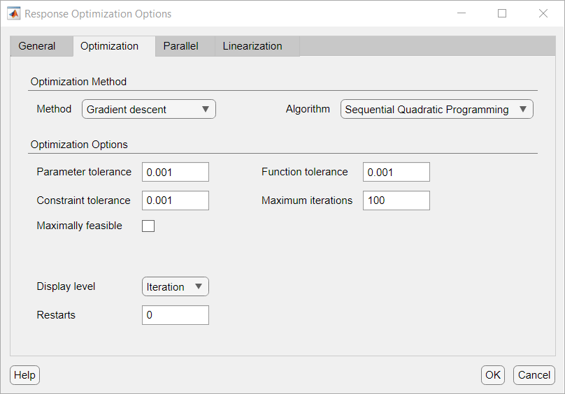
Now, try solving this optimization problem using a derivative-based solver. The optimization options can be seen by clicking the Options button in the toolstrip of the app and navigating to the Optimization pane.

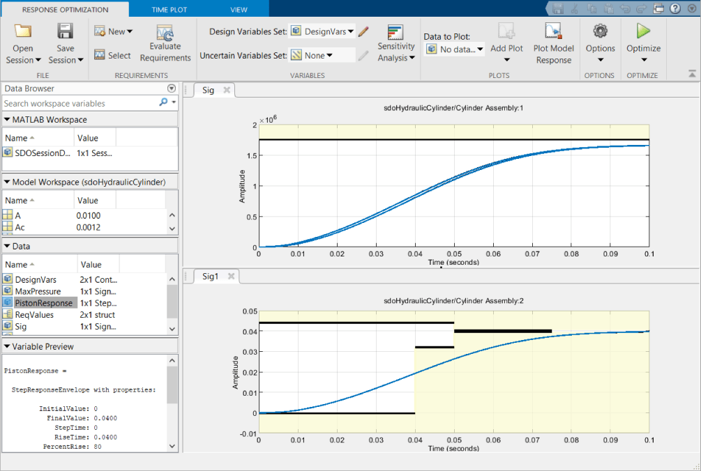
Run the optimization by clicking Optimize in the toolstrip of the app. At the end of optimization iterations, the piston response curve still goes into the yellow part of the plot, and in the numeric progress display, the bottom row of the piston response column is positive, indicating that the derivative-based solver does not satisfy all the requirements.

Optimization Options Using Surrogate Solver

Since the derivative-based solver does not satisfy all the requirements, try surrogate optimization as a derivative-free solver. Click the Options button in the toolstrip of the app and navigate to the Optimization pane. Select the surrogate optimization solver and set the maximum evaluations to 200. Click OK to use these options.

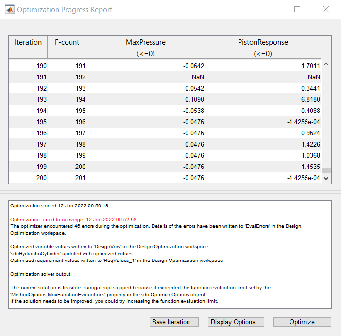
Some stages of surrogate optimization use pseudo-random number generators to select points at which to evaluate the surrogate model. For reproducible results, type rng('default') in the MATLAB® command window. Run the optimization by clicking Optimize in the toolstrip of the app. At the end of optimization, both requirements are satisfied, as seen in the curves in the plots in the app, and negative values in the bottom row of both requirement columns in the numeric progress display. The surrogate optimization solver does not have the same definitions of convergence as other solvers, and only declares that the optimization converged in cases where the objective function is designed to be minimized, and the final value of the objective function is below the objective limit in the options. The problem being solved here does not have an objective function being minimized; rather, it has requirements to be satisfied. For this problem, the optimization satisfied both of these constraint requirements.

In this example, a solver using surrogates is successful on an optimization problem while a derivative-based solver is unsuccessful. The surrogateopt solver is a global solver that tries many starting points. By using a surrogate of the model, surrogateopt needs to run the model only a moderate number of times.