Multiobjective Tradeoff Analysis of Power Grid Model

This example uses:

This example shows how to perform multiobjective tradeoff analysis of a power grid model using the Response Optimizer app.

You perform the multiobjective analysis on a Simscape™ model of an electrical power grid network with the aim to minimize the total power generated to sustain the network and to minimize the voltage deviation within the network. You then use the built-in multiobjective scatter and parallel plots to visualize the tradeoffs among the objectives, analyze trends in the Pareto-optimal designs, and select the design that best meets your specific tradeoff preferences.

IEEE 9-Bus Loadflow Model

This example explores tradeoffs for the IEEE® 9-Bus Loadflow model. This Simscape Electrical™ model is an IEEE benchmark test case [1].

For more information about this model, see IEEE 9-Bus Loadflow (Simscape Electrical).

Open the Simscape model.

open_system('sdoIEEE9BusLoadflow');

Design Problem

Tune these design parameters:

The active power generated by the G2C generator (g2cAPG).
The active power generated by the G3C generator (g3cAPG).

The design goals are:

To minimize the total active power generated to sustain the network load requirements. A lower power generation results in lower overhead and operating costs.
To minimize the voltage variation within the network. A lower voltage variation corresponds to a better quality of electric power supply that aligns with the regulatory standards.

Open Session

To launch the preconfigured tradeoff exploration session in Response Optimizer, in the model, in the Apps tab, click Response Optimizer. In the app, in the Response Optimization tab, in the Open Session menu, click Open from file and load the sdoIEEE9BusLoadflow_sdosession.mat session. You can also open the preconfigured session by directly double-clicking the Tradeoff Exploration with preloaded data block at the bottom of the Simscape model.

Define Design Variables

To view the design variables available for tuning, in the Variables section of the Response Optimization tab, click the Edit button to the right of the Design Variables Set menu. Clicking this button opens the Edit: ParamValues dialog box. You can use this parameter editor dialog to select the variables to tune as either continuous or discrete variables. You can also set their initial values and specify their respective bounds or permissible values. The app determines the scaling factor for the variables automatically.

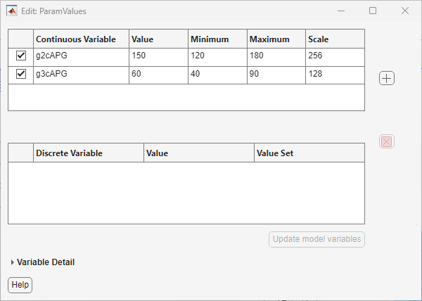
The preconfigured session is set up to tune these two continuous design variables:

The Active power generated by G2C/PV generator, denoted by g2cAPG in the model. This design variable is set up to be tuned between 120 MW to 180 MW.
The Active power generated by G3C/PV generator, denoted by g3cAPG in the model. This design variable is set up to be tuned between 40 MW to 90 MW.

Define Design Objectives as Requirements

To define the design objectives, create requirements that minimize or maximize some quantity of interest evaluated from the model. To create a requirement, use the New menu in the Requirements section of the Response Optimization tab. You can use these requirements to define objectives:

Signal Property — This requirement minimizes or maximizes one of the predefined attributes of the selected model signals.
Custom Requirement — This requirement minimizes or maximizes a custom-defined attribute of the model parameters or selected model signals.

The preconfigured session contains two requirements that correspond to the two objectives of the design problem.

TotalPowerReq — This requirement minimizes the total power generated in the network.
VoltageDeviationReq — This requirement minimizes the voltage deviation in the network.

The tradeoff exploration performed in this example does not include any constraints. However, you can perform a constrained tradeoff exploration by creating constraint requirements in addition to the objective requirements.

Define Power Generation Requirement

To view or edit the power generation requirement settings, in the Data section of the app, double-click the TotalPowerReq requirement. This requirement is a Custom Requirement that minimizes the output of the sdoCalculateTotalPower function.

To view the sdoCalculateTotalPower function, open the sdoCalculateTotalPower.m file or enter this command at the MATLAB® command prompt.

type sdoCalculateTotalPower

function vals=sdoCalculateTotalPower(data)
%TOTALPOWERREQUIREMENT
%
% The totalPowerRequirement function defines a custom requirement used in the
% graphical SDOTOOL environment.

% The |vals| return argument is the value returned to the SDOTOOL
% optimization solver.
%
% The |data| input is a structure with fields containing design variable
% values and logged simulation data. For example, if SDOTOOL is configured
% to optimize a design variable set |DesignVars| and the custom requirement
% configured to log a signal |Sig| the |data| structure has fields as
% follows:
%
% data.DesignVars    %Design variable values
% data.Nominal.Sig   %Logged signal when simulating model with |DesignVars|
%
% If SDOTOOL is configured to optimize with an uncertain variables set the
% |data| structure includes fields with logged signals when simulating the
% model with |DesignVars| and uncertain values:
%
% data.Uncertain.Sig
%
% For an example of a custom requirement function see:
% - openExample('sldo/DesignOptimizationToMeetACustomObjectiveGUIExample').
%
vals= data.DesignVars(1).Value + data.DesignVars(2).Value;
% vals= data.ParamValues(1).Value + data.ParamValues(2).Value;

end

The sdoCalculateTotalPower function returns the sum of the two design variables that govern the active power generated in the network model. Because this function relies solely on the design variables to compute the total active power generated, you do not need to log signals for the TotalPowerReq requirement

Define Voltage Deviation Requirement

To view or edit the voltage deviation requirement settings, in the Data section of the app, double-click the VoltageDeviationReq requirement. This requirement is a Custom Requirement that minimizes the output of the sdoCalculateVoltageDeviation function.

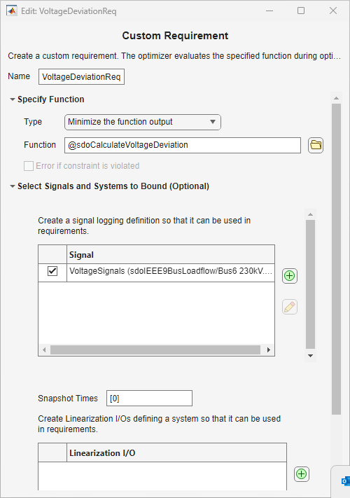
To calculate the voltage deviation, the VoltageDeviationReq requirement logs the signals in the VoltageSignals signal set and passes the logged data to the sdoCalculateVoltageDeviation function. You can add a signal to log by clicking the Add button under the Select Signals and Systems to Bound section, clicking the Simulink® signal or Simscape block of interest in the model, and selecting it in the Create Signal Set dialog box.

To view or edit the list of logged signals, in the Select Signals and Systems to Bound section, click on the VoltageSignals signal set and then click the Edit button.

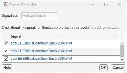
Here, the voltage deviation is calculated by logging the Voltage (Vt) output of three sampled Busbar blocks (Bus 5, Bus 6, and Bus 8) in the model. You can sample any number of Busbar blocks to calculate the voltage deviation.

To view the sdoCalculateVoltageDeviation function, open the sdoCalculateVoltageDeviation.m file or enter this command at the MATLAB command prompt.

type sdoCalculateVoltageDeviation

function vals=sdoCalculateVoltageDeviation(data)
%VOLTAGEDEVIATIONREQUIREMENT
%
% The voltageDeviationRequirement function defines a custom requirement used in the
% graphical SDOTOOL environment.

% The |vals| return argument is the value returned to the SDOTOOL
% optimization solver.
%
% The |data| input is a structure with fields containing design variable
% values and logged simulation data. For example, if SDOTOOL is configured
% to optimize a design variable set |DesignVars| and the custom requirement
% configured to log a signal |Sig| the |data| structure has fields as
% follows:
%
% data.DesignVars    %Design variable values
% data.Nominal.Sig   %Logged signal when simulating model with |DesignVars|
%
% If SDOTOOL is configured to optimize with an uncertain variables set the
% |data| structure includes fields with logged signals when simulating the
% model with |DesignVars| and uncertain values:
%
% data.Uncertain.Sig
%
% For an example of a custom requirement function see:
% - openExample('sldo/DesignOptimizationToMeetACustomObjectiveGUIExample').

deviations = abs([data.Nominal.VoltageSignals.Data]-1);
% deviations = abs(data.Nominal.VoltageSignals.Data-1);
vals = max(deviations,[],'all');
end

The sdoCalculateVoltageDeviation function calculates the deviation for all the logged signals and returns the value of the maximum deviation.

Set Up Tradeoff Exploration Problem

To open the tradeoff exploration options, in the Response Optimization tab, in the Options menu, click Tradeoff Exploration. The dialog box shows the method for tradeoff exploration, the associated stopping criteria, and other parameters.

To perform the multiobjective tradeoff exploration, the preconfigured session uses the paretosearch solver with the default tolerances. Further, the session is set up to explore 15 Pareto-optimal designs (as specified in Pareto set size) within 10 iterations (as specified in Maximum iterations). For more information about the paretosearch solver options, see options (Global Optimization Toolbox).

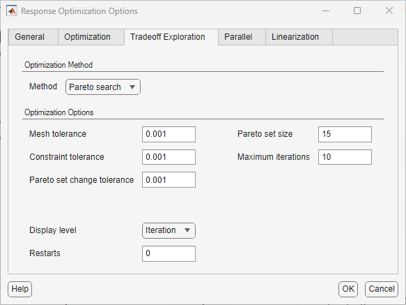
To save and close the Response Optimization Options dialog box, click OK.

Perform Tradeoff Exploration

To perform tradeoff exploration, in the app, in the Response Optimization tab, click Explore Tradeoffs. This selection launches the Optimization Progress Report dialog box and shows the status of the multiobjective optimization.

To speed up tradeoff exploration, you can use parallel computing if you have Parallel Computing Toolbox™. For more information, see Use Parallel Computing for Response Optimization.

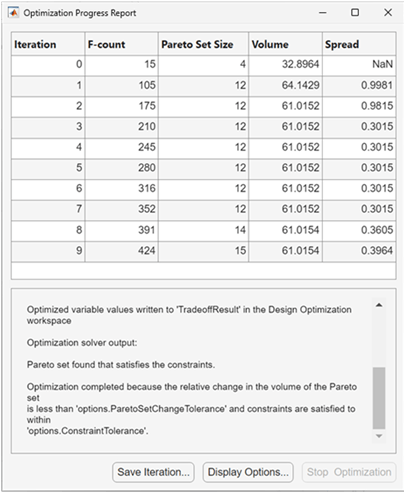
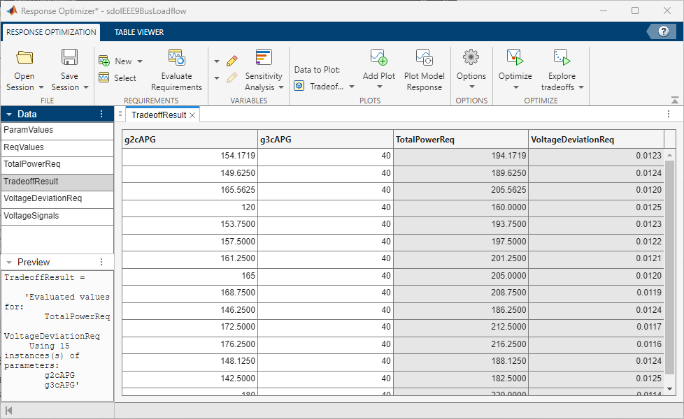
At the conclusion of the optimization session, a new entry named TradeoffResult appears in the Data section of the app. To view a table that contains the values of design variables and objectives for the identified Pareto-optimal designs, double-click TradeoffResult.

Visualize and Analyze Results

In the Response Optimization tab, in the Data to Plot menu, select TradeoffResult. To view the plots available for the selected data object, click the Add Plot menu. For a tradeoff exploration result object that consists of two or more objectives, you can use Multiobjective scatter plot and Parallel plot to perform multiobjective analysis.

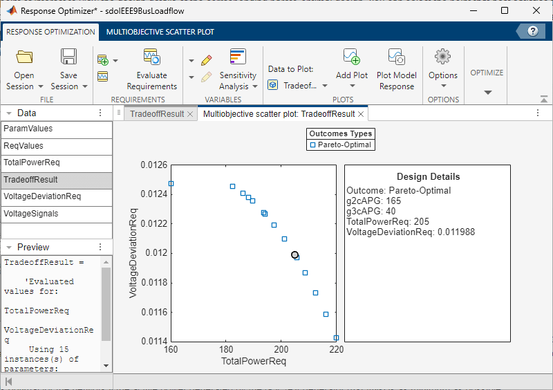
To visualize the tradeoffs between the design objectives, create a multiobjective scatter plot. To create a multiobjective scatter plot, in the Add Plot menu, click Multiobjective scatter plot. Each point on the plot represents a Pareto-optimal design identified by the paretosearch solver. The presence of the Pareto front indicates that there is a compromise between the two objectives and that no solution can simultaneously optimize both objectives.

Observe that the Pareto front is nonconvex in shape. Traditional tradeoff exploration methods, such as weighted sum aggregation of objectives, cannot typically discover such nonconvex Pareto fronts. The shape shows the trend in the compromise between the objectives. For instance, as the TotalPowerReq decreases (improves), the VoltageDeviationReq tends to increase (degrade). However, this degradation almost saturates after the TotalPowerReq decreases to 180 MW or below.

Click on a point of interest to view the design details of the corresponding Pareto-optimal design. You can select the point that best satisfies the tradeoff between the objectives. To export the parameter values corresponding to the selected design to the data browser in the app, in the Multiobjective Scatter Plot tab, click Extract selected outcome.

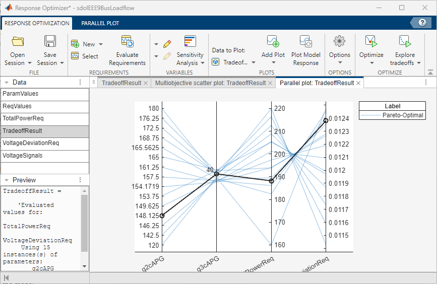
To explore trends in the Pareto-optimal designs, create a parallel plot. To do this, in the Add Plot menu, click Parallel plot. Each line on the plot represents a Pareto-optimal design identified by the paretosearch solver. You can point to a line of interest to highlight it and view its corresponding design details. Observe that all Pareto-optimal designs have g3cAPG (active power generated by G3C/PV generator) set to 40 MW, which is the lower bound of this design variable. This observation suggests that:

It is optimal for the network if the active power generated by the G3C/PV generator (g3cAPG) is as minimum as possible.
The tradeoff between the objectives is primarily governed by active power generated by the G2C/PV generator (g2cAPG). A higher value of g2cAPG results in increased total power generated in the network but reduces the voltage deviation within the network.

Close the model.

bdclose('sdoIEEE9BusLoadflow');

References

[1] Anderson, Paul M., and A. A. Fouad. Power System Control and Stability. IEEE, 2002. https://doi.org/10.1109/9780470545577.