Iterative Learning Control of a Single-Input Single-Output System
This example shows how to use both model-free and model-based iterative learning control (ILC) to improve closed-loop trajectory tracking performance of a single-input single-output (SISO) system. To implement ILC, you can use the Iterative Learning Control block from Simulink® Control Design™ software. In this example you design an ILC controller to perform a trajectory tracking for a SISO plant model, compare the model-based and model-free ILC results to a tuned PID controller, and show that an ILC controller provides a better tracking performance when augmented to a baseline controller.
Iterative Learning Control Basics
ILC is an improvement in run-to-run control. It uses frequent measurements in the form of the error trajectory from the previous batch to update the control signal for the subsequent batch run. The focus of ILC is on improving the performance of systems that execute a single, repeated operation, starting at the same initial operating condition. This focus includes many practical industrial systems in manufacturing, robotics, and chemical processing, where mass production on an assembly line entails repetition. Therefore, use ILC when you have a repetitive task or repetitive disturbances and want to use knowledge from previous iteration to improve next iteration.
In general, ILC has two variations: model free and model based. Model-free ILC requires minimum information of your plant, which makes it easier to design and implement. Model-based ILC takes advantage of the additional knowledge of the plant, which can lead to faster convergence and better performance. For more information, see Iterative Learning Control.
Examine Model
This examples provides a preconfigured Simulink® model.

Plant and Nominal Controller
The plant is a SISO, linear, discrete-time, and second-order system.
Ts = 0.01;
A = [-0.7 -0.012;1 0];
B = [1;0];
C = [1 0];
D = 0;
sys = ss(A,B,C,D,Ts);
The nominal stabilizing controller is a PI controller. To tune a PI controller, use the pidtune function.
c = pidtune(sys,"pi");When plant operation is repeating in nature, ILC control can augment baseline PID to improve the controller performance iteration after iteration.
Model-Free Iterative Learning Control
The model-free ILC method does not require prior knowledge of the system dynamics and uses proportional and derivative error feedback to update the control history. The model-free ILC update law is:
where and are referred as ILC gains.
ILC Mode
At runtime, ILC switches between two modes: control and reset. In the control mode, ILC outputs at the desired time points and measures the error between the desired reference and output . At the end of the control mode, ILC calculates the new control sequence to use in the next iteration. In the reset mode, ILC output is 0. The reset mode must be long enough such that the PI controller in this mode brings the plant back to its initial condition.

In this example, you use a generic reference signal for the purpose of illustration. Both the control and reset modes are 8 seconds long, which makes each iteration 16 seconds long. The reference signal in the control mode is a sine wave with period of 8 seconds, starting at 0. In the reset mode, the reference signal is 0, which allows the PI controller to bring the plant back to the initial operating point.
ILC Design
Load the Simulink model containing an Iterative Learning Control block in the model-free configuration.
load_system('scdmodelfreeilc');To design an ILC controller, you configure the following parameters.
Sample time and Iteration duration — These parameters determine how many control actions ILC provides in the
controlmode. If sample time is too large, ILC might not provide sufficient compensation. If sample time is too small, ILC might take too much resources, especially it might lead to large memory footprint when model-based ILC is used.ILC gains — The gains and determine how well ILC learns between iterations. If ILC gains are too big, it might make the closed-loop system unstable (robustness). If ILC gains are too small, it might lead to slower convergence (performance).
Filter time constant — The optional low-pass filter to remove control chatter which may otherwise be amplified during learning. By default it is not enabled in the ILC block.

Define the values for the ILC controller parameters sample time Ts, iteration duration Tspan, ILC gains gammaP and gammaD, and the low-pass filter time constant filter_gain.
Ts = 0.01;
Tspan = 8;
gammaP = 3;
gammaD = 0;
filter_gain = 0.25;
Simulate Model and Plot Results
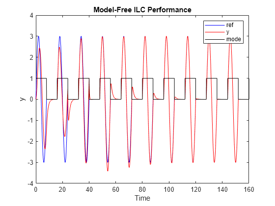
Simulate the model for 10 iterations (160 seconds). In the first iteration, ILC controller outputs 0 in the control mode because it just starts learning. Therefore, the closed-loop control performance displayed in the first iteration comes from the nominal controller, which serves as the baseline for the comparison.
simout_model_free = sim('scdmodelfreeilc');As the iterations progress, the ILC controller improves the reference tacking performance.
% Plot reference signal
figure
t = simout_model_free.logsout{6}.Values.Time;
ref = squeeze(simout_model_free.logsout{6}.Values.Data);
plot(t, ref,"b");
hold on
% Plot plant output
y = squeeze(simout_model_free.logsout{4}.Values.Data);
plot(t, y, "r");
% Plot ILC mode
mode = squeeze(simout_model_free.logsout{1}.Values.Data);
plot(t, mode,'k');
% Plot settings
xlabel('Time');
ylabel('y');
legend('ref','y','mode');
title('Model-Free ILC Performance');
hold off;
Plot the ILC and PI control efforts.
figure;
uILC = squeeze(simout_model_free.logsout{2}.Values.Data);
uPID = squeeze(simout_model_free.logsout{3}.Values.Data);
plot(t,uILC,t,uPID)
xlabel('Time')
ylabel('u');
legend('ILC','PI');
title('Model-Free ILC Control Efforts');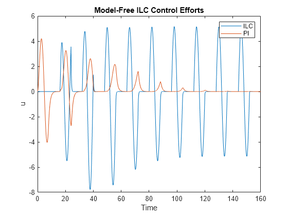
After the ILC controller learns how to compensate, the nominal PID control effort is reduced to minimum.
Model-Based Iterative Learning Control
As previously discussed, there are multiple ways to design the learning function in the ILC control law.
When you design based on the plant input-output matrix , it is called model-based ILC. Additionally, the iterative learning control block provides two types of model-based ILC: gradient based and inverse-model based.
Gradient Based ILC Law
The gradient-based ILC uses the transpose of input-output matrix in the learning function.
Therefore, ILC control law becomes , where is the ILC gain.
Inverse Model based ILC Law
The inverse model based ILC uses the inverse of input-output matrix in the learning function.
Therefore, ILC control law becomes , where is the ILC gain.
When matrix is not square, the block uses a pseudoinverse instead.
ILC Design
Load the Simulink model containing an Iterative Learning Control block in the model-based ILC configuration.
mdl = 'scdmodelbasedilc';
load_system(mdl);
Define the values for the ILC controller parameters sample time Ts, iteration duration Tspan, ILC gain gamma, and the low-pass filter time constant filter_gain.
Ts = 0.01;
Tspan = 8;
gamma = 3;
filter_gain = 0.25;

Simulation Result
Simulate the model for 10 iterations (160 seconds). In the first iteration, ILC controller outputs 0 in the control mode because it just starts learning. Therefore, the closed-loop control performance displayed in the first iteration comes from the nominal controller, which serves as the baseline for the comparison.
First, set the ILC block to use the gradient-based ILC law and simulate the model.
set_param([mdl,'/Iterative Learning Control'], 'ModelBasedILCtype','Gradient based');
simout_gradient_based = sim(mdl);
Then, set the ILC block to use the inverse-model-based ILC law and simulate the model again.
set_param([mdl,'/Iterative Learning Control'], 'ModelBasedILCtype','Inverse-model based');
simout_inverse_based = sim(mdl);
As the iterations progress, both ILC controllers improve the reference tacking performance.
% Plot reference signal
figure
t = simout_gradient_based.logsout{6}.Values.Time;
ref = squeeze(simout_gradient_based.logsout{6}.Values.Data);
plot(t, ref, 'b');
hold on
% Plot plant output controlled by gradient based ILC
y = squeeze(simout_gradient_based.logsout{4}.Values.Data);
plot(t, y, 'r');
% Plot plant output controlled by inverse-model based ILC
y = squeeze(simout_inverse_based.logsout{4}.Values.Data);
plot(t, y, 'g');
% Plot ILC mode
mode = squeeze(simout_gradient_based.logsout{1}.Values.Data);
plot(t, mode, 'k');
% Plot settings
xlabel('Time');
ylabel('y');
legend('ref','yGradient','yInverse','mode');
title('Model-Based ILC Performance');
hold off;
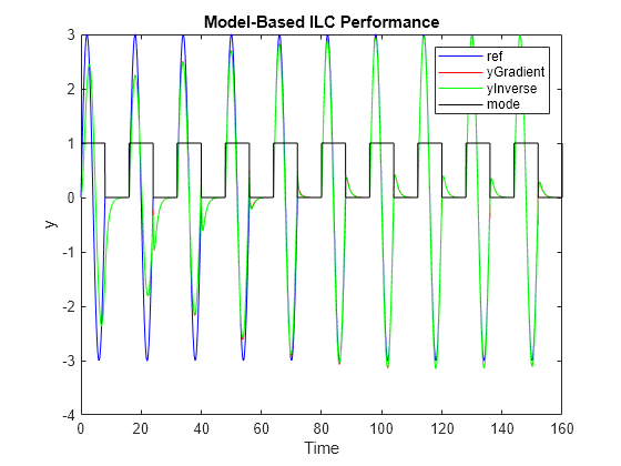
As you can observe in the preceding plot, both gradient-based ILC and inverse-model based ILC provide performance comparable to the model-free ILC in this example.