Learn and Apply Constraints for PID Controllers
This example shows how to learn constraints from data and apply these constraints for a PID control application. First, you learn the constraint function using a deep neural network, which requires Deep Learning Toolbox™ software. You then apply the constraints to the PID control actions using the Constraint Enforcement block.
For this example, the plant dynamics are described by the following equations [1].
The goal for the plant is to track the following trajectories.
For an example that applies a known constraint function to the same PID control application, see Enforce Constraints for PID Controllers.
Set the random seed and configure model parameters and initial conditions.
rng(0);           % Random seed
r = 1.5;          % Radius for desired trajectory
Ts = 0.1;         % Sample time
Tf = 22;          % Duration
x0_1 = -r;        % Initial condition for x1
x0_2 = 0;         % Initial condition for x2
maxSteps = Tf/Ts; % Simulation steps
Design PID Controllers
Before learning and applying constraints, design PID controllers for tracking the reference trajectories. The trackingWithPIDs model contains two PID controllers with gains tuned using the PID Tuner app. For more information on tuning PID controllers in Simulink® models, see Introduction to Model-Based PID Tuning in Simulink.
mdl = "trackingWithPIDs";
open_system(mdl)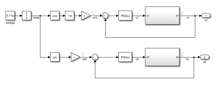
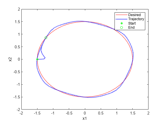
Simulate the PID controllers and plot their tracking performance.
% Simulate the model.
out = sim(mdl);

% Extract trajectories.
logData = out.logsout;
x1_traj = logData{3}.Values.Data;
x2_traj = logData{4}.Values.Data;
x1_des = logData{1}.Values.Data;
x2_des = logData{2}.Values.Data;

% Plot trajectories.
figure(Name="Tracking")
xlim([-2,2])
ylim([-2,2])
plot(x1_des,x2_des,"r")
xlabel("x1")
ylabel("x2")
hold on
plot(x1_traj,x2_traj,"b:",LineWidth=2)
hold on
plot(x1_traj(1),x2_traj(1),"g*")
hold on
plot(x1_traj(end),x2_traj(end),"go")
legend("Desired","Trajectory","Start","End", ...
    Location="best")
Constraint Function
In this example, you learn application constraints and modify the control actions of the PID controllers to satisfy these constraints.
The feasible region for the plant is given by the constraints . Therefore, the trajectories must satisfy .
You can approximate the plant dynamics by the following equation.
Applying the constraints to this equation produces the following constraint function.
The Constraint Enforcement block accepts constraints of the form . For this application, the coefficients of this constraint function are as follows.
Learn Constraint Function
For this example, the coefficients of the constraint function are unknown. Therefore, you must derive them from training data. To collect training data, use the rlCollectDataPID model. This model allows you to pass either zero or random inputs to the plant model and record the resulting plant outputs.
mdl = "rlCollectDataPID";
open_system(mdl)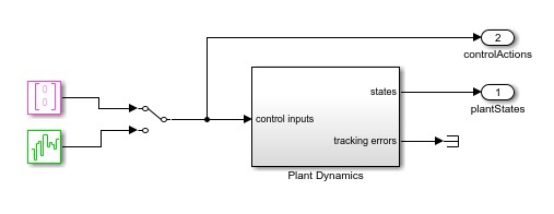
To learn the unknown matrix , set the plant inputs to zero. When you do so, the plant dynamics become .
blk = mdl + "/Manual Switch";
set_param(blk,"sw","1");
Collect training data using the collectDataPID helper function. This function simulates the model multiple times and extracts the input/output data. The function also formats the training data into an array with six columns: , , , , , and .
numSamples = 1000;
data = collectDataPID(mdl,numSamples);
Find a least-squares solution for using the input/output data.
inputData = data(:,1:2);
outputData = data(:,5:6);
A = inputData\outputData;
Collect the training data. To learn the unknown function , configure the model to use random input values that follow a normal distribution.
% Configure model to use random input data.
set_param(blk,"sw","0");

% Collect data.
data = collectDataPID(mdl,numSamples);
Train a deep neural network to approximate the function using the trainConstraintPID helper function. This function formats the data for training then creates and trains a deep neural network. Training a deep neural network requires Deep Learning Toolbox software.
The inputs to the deep neural network are the plant states. Create the input training data by extracting the collected state information.
inputData = data(:,1:2);
Since the output of the deep neural network corresponds to , you must derive output training data using the collected input/output data and the computed matrix.
u = data(:,3:4);
x_next = data(:,5:6);
fx = (A*inputData')';
outputData = (x_next - fx)./u;
Train the network using the input and output data.
network = trainConstraintPID(inputData,outputData);
    Iteration    Epoch    TimeElapsed    LearnRate    TrainingLoss    ValidationLoss
    _________    _____    ___________    _________    ____________    ______________
            0        0       00:00:00         0.01                          0.020006
            1        1       00:00:02         0.01        0.017356
           50       17       00:00:03         0.01      0.00045822        0.00054544
          100       34       00:00:03         0.01      0.00070463        0.00026694
          150       50       00:00:04         0.01      0.00028078        0.00021925
          200       67       00:00:04         0.01       0.0020676        0.00020191
          250       84       00:00:05         0.01      0.00043562         0.0001878
          300      100       00:00:05         0.01        0.002279        0.00021469
Training stopped: Max epochs completed
Save the resulting network to a MAT file.
save("trainedNetworkPID","network")
Simulate PID Controllers with Constraint Enforcement
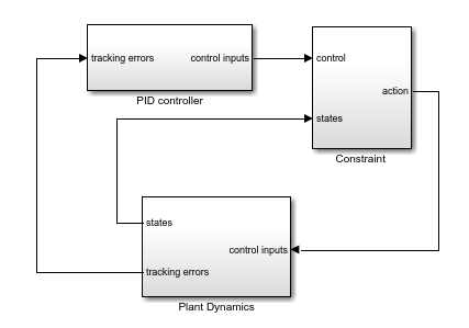
To simulate the PID controllers with constraint enforcement, use the trackingWithLearnedConstraintPID model. This model constrains the controller outputs before applying them to the plant.
mdl = "trackingWithLearnedConstraintPID";
open_system(mdl)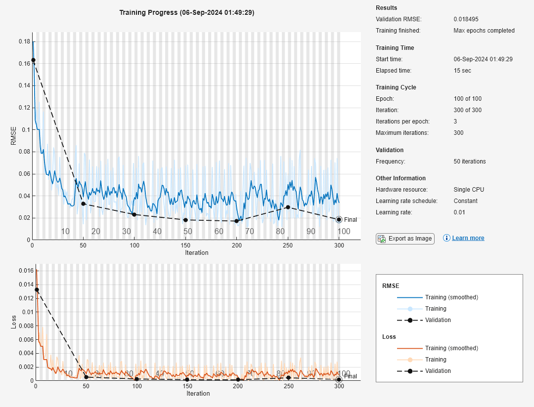
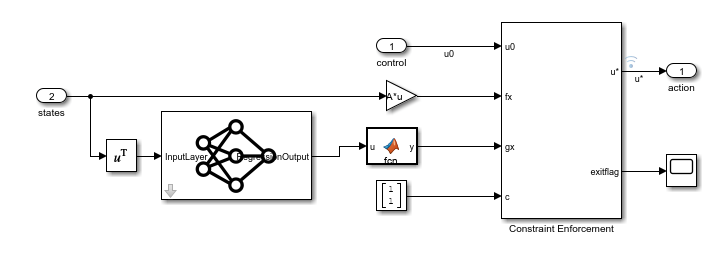
To view the constraint implementation, open the Constraint subsystem. Here, the trained deep neural network approximates based on the current plant state, and the Constraint Enforcement block enforces the constraint function.
Simulate the model and plot the results.
% Simulate the model.
out = sim(mdl);

% Extract trajectories.
logData = out.logsout;
x1_traj = zeros(size(out.tout));
x2_traj = zeros(size(out.tout));
for ct = 1:size(out.tout,1)
    x1_traj(ct) = logData{4}.Values.Data(:,:,ct);
    x2_traj(ct) = logData{5}.Values.Data(:,:,ct);
end

x1_des = logData{2}.Values.Data;
x2_des = logData{3}.Values.Data;

% Plot trajectories.
figure("Name","Tracking with Constraint");
plot(x1_des,x2_des,"r")
xlabel("x1")
ylabel("x2")
hold on
plot(x1_traj,x2_traj,"b:",LineWidth=2)
hold on
plot(x1_traj(1),x2_traj(1),"g*")
hold on
plot(x1_traj(end),x2_traj(end),"go")
legend("Desired","Trajectory","Start","End",...
    Location="best")
The Constraint Enforcement block successfully constrains the control actions such that the plant states remain less than one.
References
[1] Robey, Alexander, Haimin Hu, Lars Lindemann, Hanwen Zhang, Dimos V. Dimarogonas, Stephen Tu, and Nikolai Matni. "Learning Control Barrier Functions from Expert Demonstrations." Preprint, submitted April 7, 2020. https://arxiv.org/abs/2004.03315