Frequency Response Estimation for Power Electronics Model Using Pseudorandom Binary Signal
This example shows how to identify a frequency domain model using a pseudorandom binary sequence (PRBS) for a power electronics system modeled in Simulink® using Simscape™ Electrical™ components. This example addresses the frequency response estimation process in the controller design workflow using a PRBS as the input signal.
Typically, power electronics systems cannot be linearized because they use high-frequency switching components, such as pulse-width modulation (PWM) generators. However, most Simulink Control Design™ PID tuning tools design PID gains based on a linearized plant model. To obtain such a model for a power electronics model that cannot be linearized, you can estimate the plant frequency response over a range of frequencies, as shown in this example.
To collect frequency response data, you can:
Estimate the plant frequency response at the command line.
Estimate the plant frequency response using the Model Linearizer app.
This example shows how to estimate the plant frequency response at the command line. To learn how to estimate the plant frequency response for a power electronics system in Model Linearizer using a PRBS input signal, see Frequency Response Estimation in Model Linearizer Using Pseudorandom Binary Sequence.
Boost Converter Model
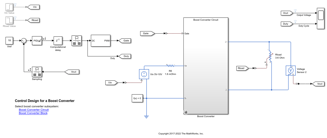
This example uses a boost converter model as a power electronics system. A boost converter circuit converts one DC voltage to another, typically higher, DC voltage by controlled chopping or switching of the source voltage.
mdl = 'scdboostconverter';
open_system(mdl)

This model uses a MOSFET driven by a PWM signal for switching. The output voltage  is regulated to the reference value
  . A digital PID controller adjusts the PWM duty cycle,
  , based on the voltage error signal. For this example, you estimate the frequency response from the PWM duty cycle to the load voltage
  .
.
Simscape Electrical software contains predefined blocks for many power electronics systems. This model contains a variant subsystem with two versions of the boost converter model:
Boost converter circuit constructed using electrical power components. The parameters of the circuit components are based on [1].
Boost converter block configured to have the same parameters as the boost converter circuit. For more information on this block, see Boost Converter (Simscape Electrical).
To use the Boost Converter block version of the subsystem, in the model, click Boost Converter Block or use the following command.
set_param([bdroot '/Boost Converter'], ...
    'LabelModeActiveChoice','block_boost_converter');
Find Model Operating Point
To estimate the frequency response for the boost converter, you must first determine the steady-state operating point at which you want the converter to operate. For more information on finding operating points, see Find Steady-State Operating Points for Simscape Models. For this example, use an operating point estimated from a simulation snapshot at 0.045 seconds.
opini = findop(mdl,0.045);
Initialize the model with the computed operating point.
set_param(mdl,'LoadInitialState','on','InitialState','getstatestruct(opini)');
Create Pseudorandom Binary Signal
A pseudorandom binary signal (PRBS) is a periodic, deterministic signal with white-noise-like properties that shifts between two values. A PRBS is an inherently periodic signal with a maximum period length of  , where
  is the PRBS order. For more information, see PRBS Input Signals.
Create a PRBS with the following configuration.
To use a nonperiodic PRBS, set the number of periods to 1.
Use a PRBS order of 14, producing a signal of length 16383. To obtain an accurate frequency response estimation, the length of the PRBS must be sufficiently large.
Set the injection frequency of the PRBS to 200 kHz to match the sample time in the model. That is, specify a sample time of
5e-6seconds.To ensure that the system is properly excited, set the perturbation amplitude to 0.05. If the input amplitude is too large, the boost converter operates in discontinuous-current mode. If the input amplitude is too small, the PRBS is indistinguishable from ripples in the power electronic circuits.
in_PRBS = frest.PRBS('Order',14,'NumPeriods',1,'Amplitude',0.05,'Ts',5e-6);
Collect Frequency Response Data
To collect frequency response data, you can estimate the plant frequency response at the command line. To do so, first get the input and output linear analysis points from the model.
io = getlinio(mdl);
Specify the operating point using the model initial conditions.
op = operpoint(mdl);
Find all source blocks in the signal paths of the linearization outputs that generate time-varying signals. Such time-varying signals can interfere with the signal at the linearization output points and produce inaccurate estimation results.
srcblks = frest.findSources(mdl,io);
To disable the time-varying source blocks, create an frestimateOptions option set and specify the BlocksToHoldConstant option.
opts = frestimateOptions;
opts.BlocksToHoldConstant = srcblks;
Estimate the frequency response using the PRBS input signal.
sysest_prbs = frestimate(mdl,io,op,in_PRBS,opts);
Analytical Transfer Function of Boost Converter Model
Analytical tranfer function can be determined based on component parameters of the model.
L = 20e-6;
C = 1480e-6;
R = 6;
rC = 8e-3;
rL = 1.8e-3;
Vo = 18;
Iload = Vo/R;
To compute the analytical transfer function, you require the actual duty cycle value. For this boost converter, use the logged duty cycle at the operating point.
D = 0.734785;
d = 1-0.734785;
Define the analytical transfer function, which is based on [1], using the component parameters in the boost converter model.
Den = [L*C*(R+rC) L+C*rL*(R+rC)+C*R*rC-R*D*C*rC R+rL-R*D-R^2*D*(1-D)/(R+rC)];
Num1 = [L/R/(1-D)^2 rL/R/(1-D)^2-R/(R+rC)+Iload/Vo*(2*rL/(1-D)^2+R*rC/(R+rC)/(1-D))];
Num = [C*rC*Num1(1) Num1(1)+C*rC*Num1(2) Num1(2)];
TFvd = tf(-R*Vo*(1-D)^2*Num, (1+rL/R/(1-D)-R*D/(R+rC))*Den);
For a more accurate description, account for the delay due to PWM signal in the transfer function TFvd.
N = 1.5;
Ts = 5e-6;
iodelay = N*Ts; % 0.5 PWM + 1 ZOH
TFvd.IODelay = iodelay;
Compare Frequency Response Data to Sinestream FRE Results
Compare the estimation results when using PRBS signal to those found using a sinestream input signal. Compare the signals across the 15 logarithmically spaced frequencies used for the sinestream ranging from 50 Hz to 5 kHz.
load frdSinestream
wbode = estsysSinestream.Frequency;
bp = bodeplot(sysest_prbs,estsysSinestream,TFvd);
bp.PhaseMatchingEnabled = "on";
bp.XLimits = [wbode(1),wbode(end)];
grid on
legend("PRBS estimation result","Sinestream estimation result", ...
"Analytical transfer function",Location="northeast");

To find the simulation time taken for frequency response estimation by an input signal, you can use the getSimulationTime function.
tfinal_sinestream = in_sine1.getSimulationTime
tfinal_prbs = in_PRBS.getSimulationTime
tfinal_sinestream =

    0.2833


tfinal_prbs =

    0.0819
The simulation time with in_PRBS is about 30% of the time taken by in_sine1 to estimate the frequency response of the model. This indicates that the frequency response estimation with PRBS input signal is much faster than the sinestream input signal.
The estimated frequency response result, sysest_prbs, closely matches estsysSinestream. Because the PRBS input signal estimates frequency responses with a large number of frequency points, the estimation result provides more information about the resonant characteristics of the system. To get similar results using sinestream input signal, you might need to increase the number of frequency points, which results in an increase in estimation time. You can use this approach to obtain accurate frequency response estimation results in a shorter simulation time as compared to estimation with sinestream signals.
Improve Frequency Response Result at Low Frequencies
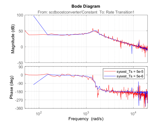
To improve the frequency response estimation result at lower frequencies, you can use a sample time slower than the sample time in the original boost converter model. To do so, modify the model to use a Constant block at the input analysis point and a Rate Transition block at the output analysis point.
For both the Constant block and the Rate Transition block, use a sample time of 5e-5 seconds, which is ten times slower than the original sample time of 5e-6 seconds.
Create a PRBS input signal using the new sample time with an order of 12.
in_PRBS = frest.PRBS('Order',12,'NumPeriods',1,'Amplitude',0.05,'Ts',5e-5);
With the new PRBS input signal, you can obtain a frequency response that extends to lower frequencies.

The ability to change the sample time of the PRBS input signal time provides an additional degree of freedom in the frequency response estimation process. Using a larger sample time than in the original model, you can obtain a higher resolution frequency response estimation result over the low-frequency range with a short simulation time. Additionally, running estimation at lower sampling rate reduces processing requirements when deploying to hardware.
References
[1] Lee, S. W. Practical Feedback Loop Analysis for Voltage-Mode Boost Converter. Application Report SLVA633. Texas Instruments, 2014. https://www.ti.com/lit/an/slva633/slva633.pdf.
See Also
frest.PRBS | frestimate | frestimateOptions