Compensate for Disturbances in Spring-Mass-Damper System

Since R2024a

This example shows how to compensate for disturbances in a spring-mass-damper system using the Disturbance Compensator block.

Spring-Mass-Damper Model

The spring-mass-damper system consists of two carts of mass ${\mathit{m}}_1$ and ${\mathit{m}}_2$, connected to each other through a spring with stiffness coefficient $\mathit{k}$ and a damper with damping coefficient $\mathit{c}$ [1].

Define the values of these physical constants in the model.

k = 1.2;
m1 = 1.5;
m2 = 1.5;
c = 1.2;

You can represent this system as a state-space model with four states $\mathit{x}=\left[\begin{array}{c}{\mathit{x}}_1\\ {\mathit{x}}_2\\ {\mathit{x}}_3\\ {\mathit{x}}_4\end{array}\right]$.

$$\begin{array}{l}\dot{\mathit{x}}={\mathit{A}}_{\mathit{p}}\mathit{x}+{\mathit{B}}_{\mathit{u}}(\mathit{u}+{\mathit{w}}_1)+{\mathit{B}}_{\mathit{d}}{\mathit{w}}_2\\ \mathit{y}={\mathit{C}}_{\mathit{p}}\mathit{x}\end{array}$$

Here:

• ${\mathit{x}}_1$ and ${\mathit{x}}_2$ are the positions of mass 1 and mass 2.

• ${\mathit{x}}_3$ and ${\mathit{x}}_4$ are the velocities of mass 1 and mass 2.

• $\mathit{u}$ is the control input acting on mass 1.

• $\mathit{y}$ is the measured output.

• ${\mathit{w}}_1$ and ${\mathit{w}}_2$ are the disturbances acting on mass 1 and mass 2.

In this example, set ${\mathit{w}}_1=0$, thus the disturbance ${\mathit{w}}_2$ and control input $\mathit{u}$ come from different channels.

Specify the state-space model for the plant ${\mathit{G}}_{\mathit{p}}$.

Ap = [0, 0, 1, 0;
      0, 0, 0, 1;
      -k/m1, k/m1, -c/m1, c/m1;
      k/m2, -k/m2, c/m2, -c/m2];
Bu = [0;0;1/m1;0];
Bd = [0;0;0;1/m2];
Cp = [0, 1, 0, 0];
Bp = [Bu,Bd];
Gp = ss(Ap,Bp,Cp,0);

Plant Knowledge for Control Design

You can approximate a mathematical model of the spring-mass-damper system by taking higher-order derivatives of $\mathit{y}$ in the dynamics equation until you find an explicit dependence on the input $\mathit{u}$. Here, the approximation is given by ${\mathit{y}}^{\left(4\right)}=\frac{\mathit{k}}{{\mathit{m}}_1{\mathit{m}}_2}\mathit{u}+\mathit{d}$, where $\mathit{d}$ represents unknown dynamics and disturbances in the system. You cannot approximate these dynamics well with a single or double integrator. Therefore, the Active Disturbance Rejection Control block is not suitable for control design and may not achieve a good performance. In this example, use the Disturbance Compensator block for satisfactory performance.

For controller design, the example considers two levels of plant knowledge.

• Minimal knowledge of plant model: ${\mathit{y}}^{\left(4\right)}=\mathit{f}\left(\mathit{t}\right)+\mathit{b}\mathit{u}$, where $\mathit{f}\left(\mathit{t}\right)$ denotes the unknown dynamics and disturbances of the system model.

• Full knowledge of plant model: $\begin{array}{l}\dot{\mathit{x}}={\mathit{A}}_{\mathit{p}}\mathit{x}+{\mathit{B}}_{\mathit{u}}\mathit{u}+{\mathit{B}}_{\mathit{d}}{\mathit{w}}_2\\ \mathit{y}={\mathit{C}}_{\mathit{p}}\mathit{x}\end{array}$.

Specify the model information for controller design with minimal plant model.

b = k/(m1*m2);
A1 = [0, 1, 0, 0;
      0, 0, 1, 0;
      0, 0, 0, 1;
      0, 0, 0, 0];
B1 = [0;0;0;b];
C1 = [1, 0, 0, 0];
sys1 = ss(A1,B1,C1,0);

Specify the model information for controller design with full plant model.

sys2 = ss(Ap,Bu,Cp,0);

Design Controller for Disturbance Compensation

First consider the case where you have full knowledge of plant model. When the variant of Disturbance Compensation is set to full knowledge, the Disturbance Compensator block is configured to have these five inports in the model.

• Nominal controller ${\mathit{u}}_0$

• Plant output $\mathit{y}$

• Disturbance input matrix ${\mathit{B}}_{\mathit{d}}$

• Observer gain matrix $\mathit{L}$

• Disturbance compensation gain ${\mathit{K}}_{\mathit{d}}$

Design a nominal state-feedback controller ${\mathit{u}}_0=\mathit{K}\hat{\mathit{x}}$ at bandwidth ${\mathit{w}}_{\mathit{c}}=1$rad/s.

wc = 1;

Specify the pole locations and differences.

dist = 1e-3;                            % pole location differences
p = -[wc,wc+dist,wc+dist*2,wc+dist*3];  % pole locations

To calculate the state-feedback matrix for both plant models, use the place command.

K2 = place(Ap,-Bu,p);                   % K2 for full knowledge of plant model
K1 = place(A1,-B1,p);                   % K1 for minimal knowledge of plant model

Design the observer gain matrix $\mathit{L}$ at bandwidth ${\mathit{w}}_{\mathit{o}}=5$ rad/s.

Specify the pole locations and spacing, extended model matrices, and use the place command to obtain the gain matrix.

wo = 5;                                         % observer bandwidth
dist = 1e-2;                                    % pole location differences
p = -[wo,wo+dist,wo+dist*2,wo+dist*3,wo+dist*4];% pole locations
Ae = [Ap,Bd;zeros(1,4),0];                      % extended model matrix 
Ce = [Cp,0];                                    % extended model matrix 
L = place(Ae',Ce',p)';                          % observer gain matrix

Compute the disturbance compensation gain ${\mathit{K}}_{\mathit{d}}$ based on [2]. For discrete-time modeling, you calculate the observer gain $\mathit{L}$ and disturbance gain $\mathit{Kd}$ matrices differently [3].

Af = Ap+Bu*K2;
Kd = -(Cp/Af*Bu)\(Cp/Af*Bd);

Open the Simulink model® with full knowledge of plant model.

mdl = 'scdSpringMassDamper';
open_system(mdl)
level = 2; % for full knowledge of plant model

Simulate the model and view the results.

out = sim(mdl);
logsout = out.logsout;
y1 = logsout.getElement('y');
y1data = y1.Values.Data(:,:)';
plot(y1.Values.Time,y1data);
xlabel('time')
ylabel('y')
grid on;
hold on;

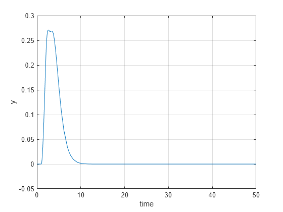
The plot shows that the disturbance is fully rejected within 10 seconds.

Compare Results

For the case where you have minimal knowledge of plant model, the linear relationship ${\mathit{B}}_{\mathit{d}}=\frac{{\mathit{m}}_1}{\mathit{k}}{\mathit{B}}_1$ holds. The Disturbance Compensator block also lets you automatically computes $\mathit{L}$ and $\mathit{Kd}$ using the block parameters. For the nominal control ${\mathit{u}}_0=\mathit{K}\hat{\mathit{x}}$, you computed the state feedback gains ${\mathit{K}}_1$ at the bandwidth ${\mathit{w}}_{\mathit{c}}=1$rad/s in the previous section. When the variant of Disturbance Compensation is set to minimal knowledge, the Disturbance Compensator block is configured to have two default inports as shown in the model.

Set controller with minimal knowledge. Simulate the model and view the results.

level = 1; % for minimal knowledge of plant model
out = sim(mdl);
logsout = out.logsout;
y2 = logsout.getElement('y');
y2data = y2.Values.Data(:,:)';
plot(y2.Values.Time,y2data);
legend('full knowledge','minimal knowledge')

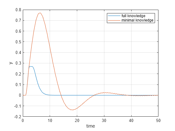
The plot shows that, for this example, more knowledge of plant model leads to better disturbance rejection performance given the same controller and observer bandwidth.

Close the model.

bdclose(mdl)

References

[1] Wie, Bong, and Dennis S. Bernstein. “Benchmark Problems for Robust Control Design.” In 1991 American Control Conference, 1929–30. Boston, MA, USA: IEEE, 1991. https://doi.org/10.23919/ACC.1991.4791727.

[2] Li, Shihua, Jun Yang, Wen-Hua Chen, and Xisong Chen. “Generalized Extended State Observer Based Control for Systems With Mismatched Uncertainties.” IEEE Transactions on Industrial Electronics 59, no. 12 (December 2012): 4792–4802. https://doi.org/10.1109/TIE.2011.2182011.

[3] Zhang, Pengcheng, Jianyu Wang, Yun Cheng, and Shiyu Jiao. “Reduced-Order Generalized Extended State Observer Based Control for Discrete-Time Systems.” In 2022 International Conference on Cyber-Physical Social Intelligence (ICCSI), 670–75. Nanjing, China: IEEE, 2022. https://doi.org/10.1109/ICCSI55536.2022.9970623.