Design Active Disturbance Rejection Control for SEPIC Converter

Since R2024a

This example shows how to design active disturbance rejection control (ADRC) for a single-ended primary-inductor converter (SEPIC) converter modeled in Simulink® using Simscape™ Electrical™ components. In this example, you also compare the ADRC control performance with a PID controller tuned on a linearized plant model.

Although you can tune the PID controller over a wide operating range, designing experiments and tuning PID gains require significant efforts. Using ADRC you can obtain a nonlinear controller and achieve better performance with a simpler setup and less tuning effort.

SEPIC Converter Model

This example uses a SEPIC converter model that converts one DC voltage to another, either higher or lower DC voltage by controlled chopping or switching of the source voltage. This model is based on the SEPIC converter model provided with Simscape Electrical software. For more information, see SEPIC Voltage Control (Simscape Electrical).

mdl = "scdSEPICConverterADRC";
open_system(mdl);

This model contains a Controller variant subsystem with three choices: an ADRC controller, a PI controller, and an open-loop control configuration with a fixed duty cycle. The open-loop control variant is useful for tuning the active disturbance rejection controller. The Active Disturbance Rejection Control subsystem is set as the default active variant.

The variant subsystem blocks take in the output voltage reference voltSEPIC_Ref and the measured output voltage voltSEPIC and output the desired duty cycle as the output to the PWM generator. For example, this image shows the configuration of the Active Disturbance Rejection Control subsystem.

The SEPIC converter model uses an ideal semiconductor switch driven by a pulse-width modulation (PWM) signal for switching. The controllers adjust the PWM duty cycle Duty, based on both the reference value and output voltage signals. The duty cycle regulates the output voltage Vout to the reference value voltRef.

Design ADRC Controller

ADRC is a powerful tool for the controller design of a plant with unknown dynamics and internal and external disturbances. The block models unknown dynamics and disturbances as an extended state of the plant and estimates them using an observer. The block lets you design a controller using only a few key tuning parameters for the control algorithm:

• Model order type (first-order or second order)

• Critical gain of the model response

• Controller and observer bandwidths

Additionally, you also specify the Time domain parameter to match the time domain of the plant model. In this example, time domain is set to discrete-time and with a sample time of 1e-5 seconds. The following sections describe how to find the remaining tuning parameters specified in the ADRC block parameters for this model.

Model Order and Critical Gain

To identify the model order, simulate the plant model with the Controller variant subsystem in the open-loop configuration. Use a step input of 0.615 as duty cycle to drive the plant model.

To switch the system to open-loop configuration, set the variant condition value.

set_param([mdl+"/Controller"],...
    "LabelModeActiveChoice","OpenLoop");

Set the name for the signal logging variable and simulate the model.

set_param(mdl,"SignalLoggingName","openLoopSim");
sim(mdl);
figure;
Ref = getElement(openLoopSim,"voltRef");
Vout = getElement(openLoopSim,"Vout");
plot(Ref.Values.Time,Ref.Values.Data...
    ,Vout.Values.Time,Vout.Values.Data)
grid on
xlim([0 0.13])
xlabel("Time (s)")
ylabel("Output Voltage (V)")
legend("Ref","Output")

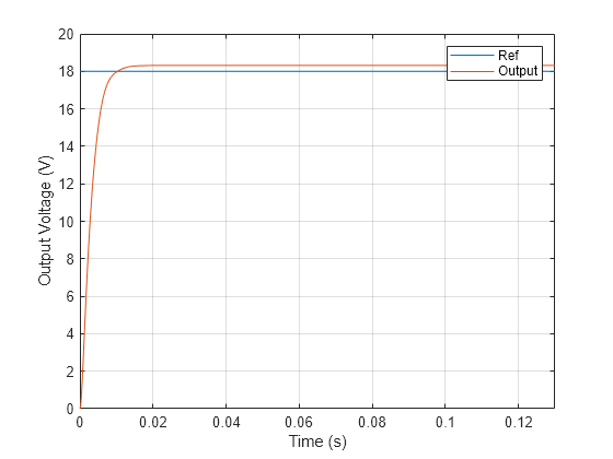
To determine the critical gain value b0, you can examine the output voltage response over a short interval of 0.0005 seconds right after the step reference input.

x = Vout.Values.Time(1:173);
y = Vout.Values.Data(1:173);
figure
plot(x,y)
xlabel("Time (s)")
ylabel("Output Voltage (V)")
grid on

Because this curve contains the effects of switching, use polyfit to get a better approximation of the output voltage over this time range.

[p,~,mu] = polyfit(x,y,3);
f = polyval(p,x,[],mu);
figure;
plot(x,y,x,f)
grid on
xlabel("Time (s)")
ylabel("Output Voltage (V)")
legend("Data","Polyfit","Location","best")

f(end)

ans = 1.0096

The output voltage shows a typical shape for a second-order dynamic system. As a result, select second-order for the Model type parameter. Based on the output voltage waveform, you can determine the critical gain

through the second-order response approximation $\mathit{y}=\frac{1}{2}\mathit{a}{\mathit{t}}^2$.

Over a duration of 0.0005 seconds, the output voltage changes by about 1.0096V.

$$a=\frac{2\mathit{y}}{{\mathit{t}}^2}=\frac{2\times 1.0096}{{\left(5{\mathit{e}}^{-4}\right)}^2}=8.0768{\mathit{e}}^6$$

$${\mathit{b}}_0=\frac{\mathit{a}}{\mathit{u}}=\frac{8.0768{\mathit{e}}^6}{0.615}=1.3133{\mathit{e}}^7$$

Controller Bandwidth and Observer Bandwidth

The controller bandwidth usually depends on the performance specifications, either in the frequency domain or time domain. In this example, the controller bandwidth ${\omega }_{\mathit{c}}$ is 500 rad/s. The observer needs to converge faster than the controller. In general, the observer bandwidth is set to 5 to 10 times ${\omega }_{\mathit{c}}$. In this example, ${\omega }_{\mathit{o}}=7\times {\omega }_{\mathit{c}}$.

Simulate Model

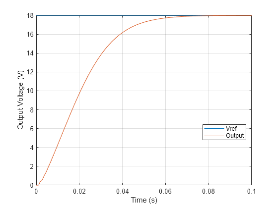
With the ADRC parameters set, run the simulation to verify if the controller tracks the output voltage reference.

set_param([mdl+"/Controller"],...
    "LabelModeActiveChoice","ADRC");
set_param(mdl,"SignalLoggingName","adrcSim");
sim(mdl);
Vref = getElement(adrcSim,"voltRef");
Vout_adrc = getElement(adrcSim,"Vout");
figure;
plot(Vref.Values.Time,Vref.Values.Data...
    ,Vout_adrc.Values.Time,Vout_adrc.Values.Data)
grid on
xlim([0 0.05])
xlabel("Time (s)")
ylabel("Output Voltage (V)")
legend("Vref","Output", "Location", "best")

Performance Comparison of ADRC and PID Controller

You can examine the tuned controller performance using a simulation with line and load disturbances. The model uses the following disturbances.

• Line disturbance at t = 0.15 sec which increase the input voltage from around 12V to 14V.

• Load disturbance at t = 0.25 sec, which decreases the load resistance from 100 ohms to 50 ohms.

You compare the output voltage of the SEPIC converter controlled using the ADRC controller with a PID controller tuned on a linear plant model obtained using frequency response estimation at the same operating point ${\mathit{V}}_{\mathrm{ref}}$ = 18 V.

Simulate the model with the PID Controller subsystem.

set_param([mdl+"/Controller"],...
    "LabelModeActiveChoice","PI");
set_param(mdl,"SignalLoggingName","pidSim");
sim(mdl);
Vout_pid = getElement(pidSim,"Vout");

Compare the performance of the two controllers.

figure;
plot(Vout_adrc.Values.Time,Vout_adrc.Values.Data...
    ,Vout_pid.Values.Time,Vout_pid.Values.Data)
grid on
xlabel("Time (s)")
ylabel("Output Voltage (V)")
legend("Vout (ADRC)","Vout (PID)", "Location","best")

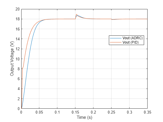
The ADRC controller drives the initial transient to the steady state much faster than the PID controller. You can further zoom in to take a closer look at how both controllers perform with the disturbances.

figure;
plot(Vout_adrc.Values.Time,Vout_adrc.Values.Data...
    ,Vout_pid.Values.Time,Vout_pid.Values.Data)
grid on
xlim([0.12 0.35])
xlabel("Time (s)")
ylabel("Output Voltage (V)")
legend("Vout (ADRC)","Vout (PID)")

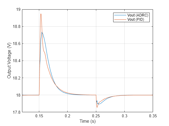
After each disturbance, the output voltage converges faster to the nominal 18 V using the ADRC controller. With an easy tuning process, the ADRC controller outperforms the tuned PID controller at the nominal operating point.

In addition, the ADRC controller works for a wide range of operating points. As a result, retuning is not necessary as with PID controllers. For example, you can compare the performance of the controllers with reference voltage of 22 V.

Set the reference voltage to 22 V and simulate the model.

set_param([mdl+"/voltRef"],"Value","22")
set_param(mdl,"SignalLoggingName","pidSim2");
sim(mdl);
Vout_pid2 = getElement(pidSim2,"Vout");
set_param(mdl,"SignalLoggingName","adrcSim2");
control=1;
set_param([mdl+"/Controller"],...
    "LabelModeActiveChoice","ADRC");
sim(mdl);
Vout_adrc2 = getElement(adrcSim2,"Vout");

Compare the performance.

figure;
plot(Vout_adrc2.Values.Time,Vout_adrc2.Values.Data...
    ,Vout_pid2.Values.Time,Vout_pid2.Values.Data)
grid on
xlabel("Time (s)")
ylabel("Output Voltage (V)")
legend("Vout (ADRC)","Vout (PID)","Location","best")

figure;
plot(Vout_adrc2.Values.Time,Vout_adrc2.Values.Data...
    ,Vout_pid2.Values.Time,Vout_pid2.Values.Data)
grid on
xlim([0.12 0.35])
xlabel("Time (s)")
ylabel("Output Voltage (V)")
legend("Vout (ADRC)","Vout (PID)")

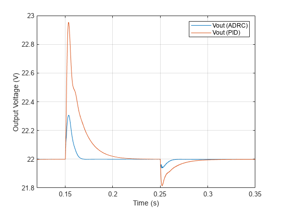
As in the previous scenario, the ADRC controller achieves faster convergence than the PID controller.

Close the model.

close_system(mdl,0);

You can set the reference voltage to values other than the original 18 V. With easy tuning, the ADRC controller performs better than the PID controller over a wide range of operating points. You can tune a PID controller to have a comparable performance as ADRC, but the process involved in tuning the gains while accounting for variations in operating conditions and external disturbances can be a tedious task.

To tune active disturbance rejection control for another power converter, see the example Design Active Disturbance Rejection Control for Boost Converter.