Handle Rate Transitions
Rate Transitions
Two periodic sample rate transitions can exist within a model:
A faster block driving a slower block
A slower block driving a faster block
The following sections concern models with periodic sample times with zero offset only. Other considerations apply to multirate models that involve asynchronous tasks. For details on how to generate code for asynchronous multitasking, see Asynchronous Support (Simulink Coder).
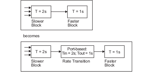
In multitasking and pseudomultitasking systems, differing sample rates can cause blocks to be executed in the wrong order. To prevent possible errors in calculated data, you must control model execution at these transitions. When connecting faster and slower blocks, you or the Simulink® engine must add Rate Transition blocks between them. Fast-to-slow transitions are illustrated in the next figure.
Slow-to-fast transitions are illustrated in the next figure.
Note
Although the Rate Transition block offers a superset of the capabilities of the Unit Delay block (for slow-to-fast transitions) and the Zero-Order Hold block (for fast-to-slow transitions), you should use the Rate Transition block instead of these blocks.
Data Transfer Problems
Rate Transition blocks deal with issues of data integrity and determinism associated with data transfer between blocks running at different rates.
Data integrity: A problem of data integrity exists when the input to a block changes during the execution of that block. Data integrity problems can be caused by preemption.
Consider the following scenario:
A faster block supplies the input to a slower block.
The slower block reads an input value V1 from the faster block and begins computations using that value.
The computations are preempted by another execution of the faster block, which computes a new output value V2.
A data integrity problem now arises: when the slower block resumes execution, it continues its computations, now using the “new” input value V2.
Such a data transfer is called unprotected. Fast-to-Slow Periodic Rate Transitions During Generated Code Execution (Simulink Coder) shows an unprotected data transfer.
In a protected data transfer, the output V1 of the faster block is held until the slower block finishes executing.
Deterministic versus nondeterministic data transfer: In a deterministic data transfer, the timing of the data transfer is completely predictable, as determined by the sample rates of the blocks.
The timing of a nondeterministic data transfer depends on the availability of data, the sample rates of the blocks, and the time at which the receiving block begins to execute relative to the driving block.
You can use the Rate Transition block to protect data transfers in your application and make them deterministic. These characteristics are considered desirable in most applications. However, the Rate Transition block supports flexible options that allow you to compromise data integrity and determinism in favor of lower latency. The next section summarizes these options.
Data Transfer Assumptions
When processing data transfers between tasks, the code generator makes these assumptions:
Data transitions occur between a single reading task and a single writing task.
A read or write of a byte-sized variable is atomic.
When two tasks interact through a data transition, only one of them can preempt the other.
For periodic tasks, the faster rate task has higher priority than the slower rate task; the faster rate task preempts the slower rate task.
All tasks run on a single processor. Time slicing is not allowed.
Processes do not crash or restart (especially while data is transferred between tasks).
Rate Transition Block Options
Several parameters of the Rate Transition block are relevant to its use in code generation for real-time execution, as discussed below. For a complete block description, see Rate Transition.
The Rate Transition block handles periodic (fast to slow and slow to fast) and asynchronous transitions. When inserted between two blocks of differing sample rates, the Rate Transition block automatically configures its input and output sample rates for the type of transition; you do not need to specify whether a transition is slow-to-fast or fast-to-slow (low-to-high or high-to-low priorities for asynchronous tasks).
The critical decision you must make in configuring a Rate Transition block is the choice of data transfer mechanism to be used between the two rates. Your choice is dictated by considerations of safety, memory usage, and performance. As the Rate Transition block parameter dialog box in the next figure shows, the data transfer mechanism is controlled by two options.
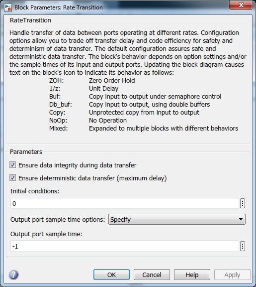
Ensure data integrity during data transfer: When you select this parameter, data transferred between rates maintains its integrity (the data transfer is protected). When you clear this parameter, data might not maintain its integrity (the data transfer is unprotected). By default, parameter Ensure data integrity during data transfer is selected.
Ensure deterministic data transfer (maximum delay): This parameter is supported for periodic tasks with an offset of zero and fast and slow rates that are multiples of each other. When this parameter is selected, the Rate Transition block behaves like a Zero-Order Hold block (for fast to slow transitions) or a Unit Delay block (for slow to fast transitions). The Rate Transition block controls the timing of data transfer in a completely predictable way. When this parameter is cleared, the data transfer is nondeterministic. By default, Ensure deterministic data transfer (maximum delay) is selected for transitions between periodic rates with an offset of zero; for asynchronous transitions, it cannot be selected.
The Rate Transition block offers three modes of operation with respect to data transfer. In order of level of safety:
Protected/Deterministic (default): This is the safest mode. The drawback of this mode is that it introduces deterministic latency into the system for the case of slow-to-fast periodic rate transitions. For that case, the latency introduced by the Rate Transition block is one sample period of the slower task. For the case of fast-to-slow periodic rate transitions, the Rate Transition block does not introduce additional latency.
Protected/NonDeterministic: In this mode, for slow-to-fast periodic rate transitions, data integrity is protected by double-buffering data transferred between rates. For fast-to-slow periodic rate transitions, a semaphore flag is used. The blocks downstream from the Rate Transition block use the latest available data from the block that drives the Rate Transition block. Maximum latency is less than or equal to one sample period of the faster task.
The drawbacks of this mode are its nondeterministic timing. The advantage of this mode is its low latency.
Unprotected/NonDeterministic: This mode is not recommended for mission-critical applications. The latency of this mode is the same as for Protected/NonDeterministic mode, but memory requirements are reduced since neither double-buffering nor semaphores are required. That is, the Rate Transition block does nothing in this mode other than to pass signals through; it simply exists to notify you that a rate transition exists (and can cause generated code to compute incorrect answers). Selecting this mode, however, generates the least amount of code.
Note
In unprotected mode (Ensure data integrity during data transfer is selected), the Rate Transition block does nothing other than allow the rate transition to exist in the model.
Rate Transition Blocks and Continuous Time
The sample time at the output port of a Rate Transition block can only be discrete or fixed in minor time step. This means that when a Rate Transition block inherits continuous sample time from its destination block, it treats the inherited sample time as Fixed in Minor Time Step. Therefore, the output function of the Rate Transition block runs only at major time steps. If the destination block sample time is continuous, Rate Transition block output sample time is the base rate sample time (if solver is fixed-step), or zero-order-hold-continuous sample time (if solver is variable-step).
Automatic Rate Transition
The Simulink engine can detect mismatched rate transitions in a multitasking model during an update diagram and automatically insert Rate Transition blocks to handle them. To enable this, select model configuration parameter Automatically handle rate transition for data transfer. By default, this parameter is cleared. When you select this parameter:
Simulink handles transitions between periodic sample times and asynchronous tasks.
Simulink inserts hidden Rate Transition blocks in the block diagram.
The code generator produces code for the Rate Transition blocks that were automatically inserted. This code is identical to the code generated for Rate Transition blocks that were inserted manually.
Automatically inserted Rate Transition blocks operate in protected mode for periodic tasks and asynchronous tasks. You cannot alter this behavior. For periodic tasks, automatically inserted Rate Transition blocks operate with the level of determinism specified by model configuration parameter Deterministic data transfer. The default setting is
Whenever
                            possible
, which enables determinism for data transfers between periodic sample-times that are related by an integer multiple. For more information, see Deterministic data transfer. To use other modes, you must insert Rate Transition blocks and set their modes manually.
For example, in this model, SineWave2 has a sample time of 2, and SineWave3 has a sample time of 3.
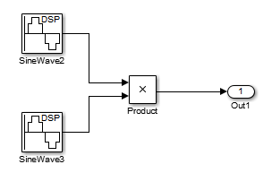
When you select model configuration parameter Automatically handle rate transition for data transfer, Simulink inserts a Rate Transition block between each Sine Wave block and the Product block. The inserted blocks have the parameter values to reconcile the Sine Wave block sample times.
If the input port and output port data sample rates in a model are not multiples of each other, Simulink inserts a Rate Transition block whose sample rate is the greatest common divisor (GCD) of the two rates. If no other block in the model contains this new rate, an error occurs during simulation. In this case, you must insert a Rate Transition block manually.
Visualize Inserted Rate Transition Blocks
When you select model configuration parameter Automatically handle rate
transition for data transfer, Simulink inserts Rate Transition blocks in the paths that have mismatched
transition rates. These blocks are hidden by default. To visualize the inserted
blocks, update the diagram. Badge labels appear in the model and indicate where
Simulink inserted Rate Transition blocks during the compilation phase. For
example, in this model, three Rate Transition blocks were inserted between the two
Sine Wave blocks and the Multiplexer and Integrator when the model compiled. The
ZOH and DbBuf badge labels indicate these blocks.
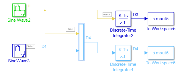
You can show or hide badge labels. Open the Debug tab. In the Diagnostics section of the Information Overlays/Sample Time gallery select or clear Automatic Rate Transitions.
To configure the hidden Rate Transition blocks so that the blocks are visible, right-click a badge label and click Insert rate transition block.
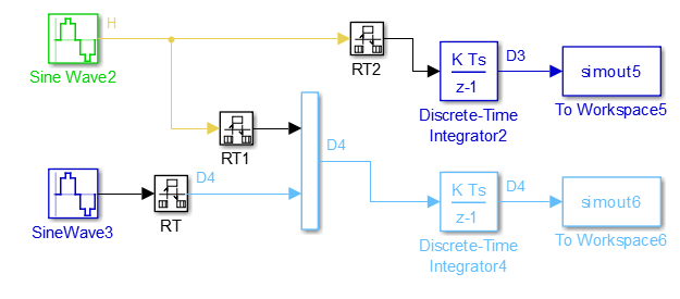
When you make hidden Rate Transition blocks visible:
You can see the type of Rate Transition block inserted and the location of the block in the model.
You can set the block parameter Initial Conditions.
You can change block parameter settings for rate transfer.
Validate the changes to your model by updating your diagram.
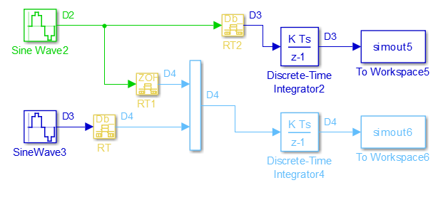
Displaying inserted Rate Transition blocks is not compatible with export-function models.
To learn more about the types of Rate Transition blocks, see Rate Transition.
Periodic Sample Rate Transitions
These sections describe cases in which Rate Transition blocks are required for periodic sample rate transitions. The discussion and timing diagrams in these sections are based on the assumption that the Rate Transition block is used in its default (protected/deterministic) mode. Model configuration parameters Ensure data integrity during data transfer and Ensure deterministic data transfer (maximum delay) are selected. These are the settings used for automatically inserted Rate Transition blocks.
Faster to Slower Transitions in a Simulink Model
In a model where a faster block drives a slower block having direct feedthrough, the outputs of the faster block are computed first. In simulation intervals where the slower block does not execute, the simulation progresses more rapidly because there are fewer blocks to execute. The next figure illustrates this situation.
A Simulink simulation does not execute in real time, which means that it is not bound by real-time constraints. The simulation waits for, or moves ahead to, whatever tasks are required to complete simulation flow. The actual time interval between sample time steps can vary.
Faster to Slower Transitions in Real Time
In models where a faster block drives a slower block, you must compensate for the fact that execution of the slower block might span more than one execution period of the faster block. This means that the outputs of the faster block can change before the slower block has finished computing its outputs. The next figure shows a situation in which this problem arises (T = sample time). Note that lower priority tasks are preempted by higher priority tasks before completion.
In the above figure, the faster block executes a second time before the slower block has completed execution. This can cause unpredictable results because the input data to the slow task is changing. Data might not maintain its integrity in this situation.
To avoid this situation, the Simulink engine must hold the outputs of the 1 second (faster) block until the 2 second (slower) block finishes executing. The way to accomplish this is by inserting a Rate Transition block between the 1 second and 2 second blocks. The input to the slower block does not change during its execution, maintaining data integrity.
It is assumed that the Rate Transition block is used in its default (protected/deterministic) mode.
The Rate Transition block executes at the sample rate of the slower block, but with the priority of the faster block.
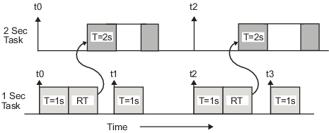
When you add a Rate Transition block, the block executes before the 2 second block (its priority is higher) and its output value is held constant while the 2 second block executes (it executes at the slower sample rate).
Slower to Faster Transitions in a Simulink Model
In a model where a slower block drives a faster block, the Simulink engine again computes the output of the driving block first. During sample intervals where only the faster block executes, the simulation progresses more rapidly.
The next figure shows the execution sequence.
As you can see from the preceding figures, the Simulink engine can simulate models with multiple sample rates in an efficient manner. However, a Simulink simulation does not operate in real time.
Slower to Faster Transitions in Real Time
In models where a slower block drives a faster block, the generated code assigns the faster block a higher priority than the slower block. This means the faster block is executed before the slower block, which requires special care to avoid incorrect results.
This timing diagram illustrates two problems:
Execution of the slower block is split over more than one faster block interval. In this case the faster task executes a second time before the slower task has completed execution. This means the inputs to the faster task can have incorrect values some of the time.
The faster block executes before the slower block (which is backward from the way a Simulink simulation operates). In this case, the 1 second block executes first; but the inputs to the faster task have not been computed. This can cause unpredictable results.
To eliminate these problems, you must insert a Rate Transition block between the slower and faster blocks.

It is assumed that the Rate Transition block is used in its default (protected/deterministic) mode.
The next figure shows the timing sequence that results with the added Rate Transition block.
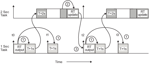
Three key points about transitions in this diagram (refer to circled numbers):
The Rate Transition block output runs in the 1 second task, but at a slower rate (2 seconds). The output of the Rate Transition block feeds the 1 second task blocks.
The Rate Transition update uses the output of the 2 second task to update its internal state.
The Rate Transition output in the 1 second task uses the state of the Rate Transition that was updated in the 2 second task.
The first problem is addressed because the Rate Transition block is updating at a slower rate and at the priority of the slower block. The input to the Rate Transition block (which is the output of the slower block) is read after the slower block completes executing.
The second problem is addressed because the Rate Transition block executes at a slower rate and its output does not change during the computation of the faster block it is driving. The output portion of a Rate Transition block is executed at the sample rate of the slower block, but with the priority of the faster block. Since the Rate Transition block drives the faster block and has effectively the same priority, it is executed before the faster block.
Note
This use of the Rate Transition block changes the model. The output of the slower block is now delayed by one time step compared to the output without a Rate Transition block.
Protect Data Integrity with volatile Keyword
When you select model configuration parameter Ensure data integrity during data transfer, the code generated for a Rate Transition block defines global buffers and semaphores and uses them to protect the integrity of the transferred data.
Particularly for a multitasking application, the tasks (rates) involved in a data
transfer can write to the transferred data, buffers, and semaphores at times that
your compiler cannot anticipate. To prevent your compiler from optimizing the
assembly code in a manner that compromises the integrity of the transferred data,
the code generator applies the keyword volatile to the buffers
and semaphores. The code generator does not apply volatile to the
global variable that represents the transferred data because the
volatile buffers and semaphores typically offer enough
protection.
With Embedded Coder®, you can explicitly apply volatile to the
transferred data by applying the built-in custom storage class
Volatile to the input of the Rate Transition
block. For example, you can use this technique to help protect the integrity of data
that your external code shares with the generated code.
Alternatively, to protect data that your external code shares with the generated
code, you can write your own C functions that read and write the data in a protected
manner. Then, you can apply the custom storage class GetSet to
the data in the model, which causes the generated code to call your functions
instead of directly accessing the data.
For more information about applying volatile, see Protect Global Data with const and volatile Type Qualifiers (Embedded Coder). For more information about GetSet, see Access Data Through Functions with Storage Class GetSet (Embedded Coder).