trim
Find trim point of dynamic system
The trim function provides only basic trimming functionality. For
full trimming functionality, use Simulink®
Control Design™ software. For more information, see Compute Steady-State Operating Points (Simulink Control Design).
Syntax
Description
The trim function starts from an initial point and
searches using a sequential quadratic programming algorithm until it finds the nearest
trim point.
You must supply the initial point implicitly or explicitly. If the
trim function cannot find a trim point, the function returns
the point encountered in its search where the state derivatives are closest to zero in a
min-max sense. In other words, the function returns the point that minimizes the maximum
deviation from zero of the derivatives. The trim function can find
trim points that meet specific input, output, or state conditions, and the function can
find points where a system is changing in a specified manner, that is, points where the
system state derivatives equal specific nonzero values.
Caution
When you use the trim function to find a trim point near a
specified initial operating point, the trim function returns
only a local value. Other, more suitable trim points might exist. To find the most
suitable trim point for a particular application, as a best practice, try a number
of initial guesses for the initial state, input, and output values.
[
finds the equilibrium point of the model specified by x,u,y,dx] = trim(sys)sys
nearest to the initial state, x0. Specifically, the
trim function finds the equilibrium point that minimizes
the maximum absolute value of [x-x0,u,y]. If
trim cannot find an equilibrium point near the system's
initial state, it returns the point at which the system is nearest to equilibrium.
Specifically, it returns the point that minimizes abs(dx), where
dx represents the derivative of the system. You can obtain
x0 using this command: [sizes,x0,xstr] =
sys([],[],[],0).
[
finds the trim point closest to x,u,y,dx] = trim(sys,x0,u0,y0,ix,iu,iy)x0, u0,
y0 that satisfies a specified set of state, input, and/or
output conditions. The integer vectors ix,
iu, and iy select the values in
x0, u0, and y0
that must be satisfied. If the trim function cannot find an
equilibrium point that satisfies the specified set of conditions exactly, it returns
the nearest point that satisfies the conditions, namely, abs([x(ix)-x0(ix);
u(iu)-u0(iu); y(iy)-y0(iy)]).
[
finds specific nonequilibrium points, that is, points at which the system's state
derivatives have some specified nonzero value. Here, x,u,y,dx] = trim(sys,x0,u0,y0,ix,iu,iy,dx0,idx)dx0
specifies the state derivative values at the search's starting point and
idx selects the values in dx0 that the
search must satisfy exactly.
[
specifies an array of optimization parameters that the x,u,y,dx,options] = trim(sys,x0,u0,y0,ix,iu,iy,dx0,idx,options)trim
function passes to the optimization function that it uses to find trim points. The
optimization function, in turn, uses this array to control the optimization process
and to return information about the process. The trim function
returns the options array at the end of the search process. By
exposing the underlying optimization process in this way, the
trim function allows you to monitor and fine-tune the
search for trim points.
Examples
Open the example model named EquilibriumPoints that models a linear state-space system by using a State-Space block.
sys = "EquilibriumPoints";
open_system(sys)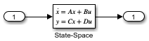
The State-Space block specifies these matrices:
A = [-0.09 -0.01;1 0]B = [0 -7;0 -2]C = [0 2;1 -5]D = [-3 0; 1 0]
To find an equilibrium point in the model, call the trim function and specify only the model name as an input argument.
[x,u,y,dx,options] = trim(sys)
x = 2×1

     0
     0
u = 2×1

     0
     0
y = 2×1

     0
     0
dx = 2×1

     0
     0
options = 1×18

         0    0.0001    0.0001    0.0000         0         0    1.0000         0         0    7.0000    2.0000         0    2.0000  500.0000         0    0.0000    0.1000    1.0000
The Simulink® trim function uses a model to determine steady-state points of a dynamic system that satisfy specified input, output, and state conditions.
Open the example model named SteadyStatePoints.
sys = "SteadyStatePoints";
open_system(sys)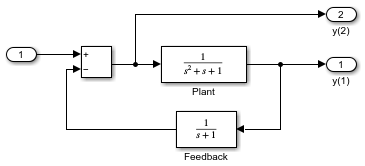
To find the values of the input and the states that result in a value of 1 for both output values, use the trim function.
Create variables named x and u to store values that represent initial guesses of the state variable values and input values, respectively. Then, create a variable named y to store the desired output value.
x = [0; 0; 0];
u = 0;
y = [1; 1];
Create index variables to specify which variables are fixed and which can vary. To specify that the state and input values can vary, assign an empty matrix ([]) to the index variables ix and iu. To specify that the output values are fixed, specify the value of the index variable iy as [1;2].
ix = [];      % Don't fix any of the states
iu = [];      % Don't fix the input
iy = [1;2];   % Fix both output 1 and output 2
To find the values of states and inputs that result in the desired output value, call the trim function. The values the trim function returns might differ due to rounding error.
[x,u,y,dx] = trim(sys,x,u,y,ix,iu,iy)
x = 3×1

    0.0000
    1.0000
    1.0000
u =
2
y = 2×1

    1.0000
    1.0000
dx = 3×1
10-15 ×

    0.2220
    0.1870
         0
Equilibrium point problems might not have a solution. In that case, the trim function first tries setting the derivatives to 0 and then returns a solution that minimizes the maximum deviation from the desired result.
Open the example model named EquilibriumPoints that models a linear state-space system by using a State-Space block.
sys = "EquilibriumPoints";
open_system(sys)
The State-Space block specifies these matrices:
A = [-0.09 -0.01;1 0]B = [0 -7;0 -2]C = [0 2;1 -5]D = [-3 0; 1 0]
To find an equilibrium point near an operating point defined by state and input values, call the trim function and specify additional input arguments that contain the state and input values to define the operating point.
x0 = [1;1];
u0 = [1;1];
[x,u,y,dx,options] = trim(sys,x0,u0)
x = 2×1
10-13 ×

   -0.2337
   -0.2353
u = 2×1

    0.3333
   -0.0000
y = 2×1

   -1.0000
    0.3333
dx = 2×1
10-13 ×

    0.8233
   -0.0051
options = 1×18

         0    0.0001    0.0001    0.0000         0         0    1.0000    1.0000         0   31.0000    6.0000         0    2.0000  500.0000         0    0.0000    0.1000    1.0000
Check the options return argument to see the number of iterations required to identify the equilibrium point near the specified operating point.
options(10)
ans =
31
To find an equilibrium point at which both output values are fixed, specify additional input arguments to indicate the target output value and that the output values are fixed.
y = [1;1];
iy = [1;2];
[x,u,y,dx] = trim(sys,[],[],y,[],[],iy)
x = 2×1

    0.0009
   -0.3075
u = 2×1

   -0.5383
    0.0004
y = 2×1

    1.0000
    1.0000
dx = 2×1
10-16 ×

    0.0043
    0.4196
To find an equilibrium point with specified derivative values at which both outputs are fixed, specify additional input arguments for the derivative values, the target output value, and that the output values are fixed.
y = [1;1];
iy = [1;2];
dx = [0;1];
idx = [1;2];
[x,u,y,dx,options] = trim(sys,[],[],y,[],[],iy,dx,idx)
x = 2×1

    0.9752
   -0.0827
u = 2×1

   -0.3884
   -0.0124
y = 2×1

    1.0000
    1.0000
dx = 2×1

   -0.0000
    1.0000
options = 1×18

         0    0.0001    0.0001    0.0000         0         0    1.0000         0         0   13.0000    3.0000         0    2.0000  500.0000         0    0.0000    0.1000    1.0000
Check the options return argument to see the number of iterations required to identify the equilibrium point near the specified operating point.
options(10)
ans =
13
Input Arguments
Output Arguments
More About
Algorithms
The trim function uses a sequential quadratic programming
algorithm to find trim points. For a description of this algorithm, see Sequential Quadratic Programming (SQP) (Optimization Toolbox).
Version History
Introduced before R2006a
See Also
findop (Simulink Control Design)
Topics
- Compute Steady-State Operating Points (Simulink Control Design)