Simulink Simulation
Simulating the model of a dynamic system allows you to gain insight about the behavior of a proposed system design without the time consuming process of actually building the system. The concepts in this topic provide a context for understanding how to control a model simulation with Simulink® software tools.
Compilation
Compilation is the Simulink process where the block diagram is translated to an internal representation that interacts with the Simulink engine.
There are no model-level sets of differential equations that are solved numerically as a whole. Instead, the model-level equations correspond to the individual block equations that are solved numerically in a specific order.
Block Methods
The functionality of a single block is defined by multiple equations. These equations are represented as block methods. These block methods are evaluated (executed) during the execution of a block diagram. The evaluation of these block methods is performed within a simulation loop, where each cycle through the simulation loop represent the evaluation of the block diagram at a given point in time. Common block methods include:
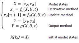
Derivative – Computes the derivatives of the block's continuous states at the current time step, given the block inputs and the values of the states at the previous time step.
Update – Computes the value of the block's discrete states at the current time step, given its inputs at the current time step and its discrete states at the previous time step.
Output – Computes the outputs of a block given its inputs at the current time step and its states at the previous time step.
Model Method
In addition to block methods, a set of methods is provided that compute the model properties and its outputs. The Simulink software similarly invokes these methods during simulation to determine a model's properties and its outputs. The model methods generally perform their tasks by invoking block methods of the same type. For example, the model Outputs method invokes the Outputs methods of the blocks that it contains in the order specified by the model to compute its outputs. The model Derivatives method similarly invokes the Derivatives methods of the blocks that it contains to determine the derivatives of its states.
See also: Simulation Phases in Dynamic Systems.
Callback
Callbacks are MATLAB® expressions that execute in response to a specific modeling action. Simulink provides model, block, and port callback parameters that identify specific kinds of modeling actions. You provide the code for callback parameters. Simulink executes the callback code when the associated modeling action occurs.
Model Callback
Model callback parameters include:
PreloadFcn– Executes before a model loads. For example, you can provide code that loads the variable values a model uses into the MATLAB workspace.
See Model Callbacks.
Block Callback
Block callback parameters include:
OpenFcn– Execute when you open a Subsystem block.LoadFcn– Execute after a diagram is loaded. For a Subsystem blocks, also execute block callback parameters for the blocks within Subsystem block.
Port Callback
Port callback parameter:
ConnectionCallback- Execute code every time the connectivity of a port changes.
See Port Callbacks.
Execution Order
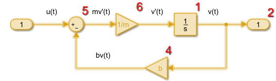
The Execution order is the sequence in which block output methods are called after evaluating direct feedthrough of each input port. To display execution order, in the Debug tab, select Information Overlays > Execution Order.
In the following model, the Integrator block output runs first, and then the loop of blocks connected to the Integrator block input. Missing execution numbers in a sequence are usually due to so-called "hidden buffer" blocks; see Ensure Output Port Is Virtual.
See also: Control and Display Execution Order, Simulation Phases in Dynamic Systems.
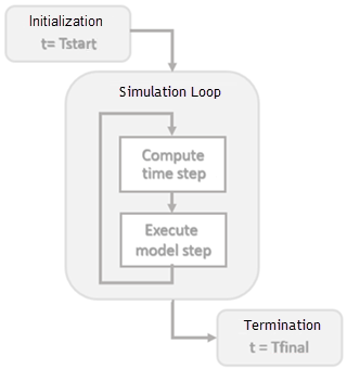
Simulation
Simulation is the process after model compilation where block method outputs and states are computed at successive time steps over a specified time range using a numerical solver.
During each simulation loop, Simulink calculates a Δt to determine the time step
t(k+1) = t(k) + Δt. The size of Δt is based on
an estimated error between the simulated solution and the actual solution. At the end of
a simulation, data results are given as vectors [t, X, Y] for time,
state and output at each time step.
See also: Simulation Phases in Dynamic Systems, Simulate a Model Interactively, Speed Up Simulation.
Solver
A Solver finds an approximate solution for a set of model equations. Simulink uses established numerical solvers for this task.
Solver step size can be fixed or variable:
Fixed step – Time step
T(k+1) = T(k) + ΔtwhereΔtis constant. If step size is too large, simulation results can have a large error. In the following example, a step size of2distorts the shape of a sine wave signal. You can specify the size of the time step in the case of fixed-step solvers, or the solver can automatically determine the step size in the case of variable-step solvers.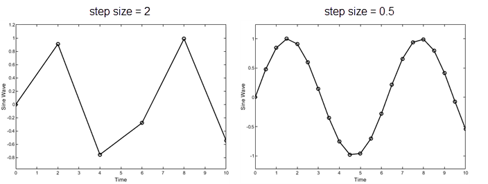
Variable step – Variable step solvers iterate to reach a solution based on an error tolerance. Time step
T(k+1) = T(k) + ΔtₖwhereΔtₖchanges from one simulation step to the next depending on the estimated error. Smaller time steps increase the accuracy of the simulation results. To minimize the computation workload, a variable-step solver chooses the largest step size consistent with achieving an overall level of precision specified by the error tolerance and observing zero-crossings. This ensures that all model states are computed to the accuracy specified by the user.
Choosing a solver method depends on the nature of the model equations. Euler's method
is a simple numerical solver that calculates the next value of y by
using the slope (y') of a tangent line to y. If
y is a function that integrates a ramp function x with a slope of
1, y' = x, and a numerical solver would use the following
equations.
x[n+1] = x[n] + Δt*1
y[n+1] = y[n] + Δt*x[n+1]
Decreasing the step size increases the accuracy of the results. but it increases the
time to complete a simulation. In the following example, a step size of
2 shows an error of about 20 percent after 10 seconds while a
step size of 0.5 produces a result that is closer to the actual
solution.
