Run Parameter Sweep Using Parallel Simulations
This example shows how to run multiple simulations of a Monte Carlo study in parallel using parsim and Parallel Computing Toolbox™. Parallel execution leverages the multiple cores of your host machine to speed up multiple simulations. These simulations can also be run in parallel on compute clusters using MATLAB® Parallel Server™. If you do not have Parallel Computing Toolbox or MATLAB Parallel Server, the simulations in this example run serially.
Explore Model
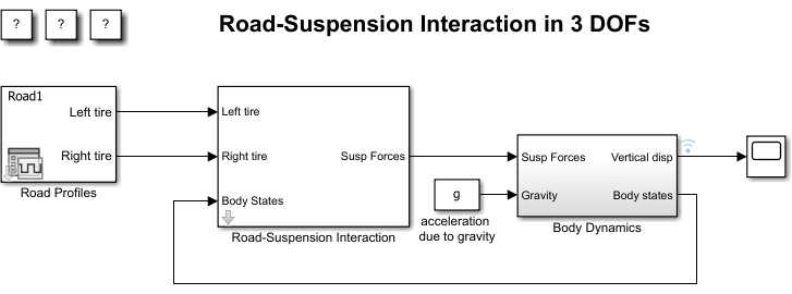
The model sldemo_suspn_3dof simulates vehicle dynamics based on the interaction between the road and the vehicle suspension for different road profiles. The model captures vehicle dynamics in three degrees of freedom: vertical displacement, roll, and pitch. The Signal Editor block named Road Profiles stores measured road profile data for the left and right tires as different test groups. The Road-Suspension Interaction subsystem calculates the suspension forces on the vehicle at the four tire locations based on the road data and the current vehicle state. The Body Dynamics subsystem uses these forces and the resulting pitch and roll moments to calculate the vehicle motion in each of the three degrees of freedom.
mdl = "sldemo_suspn_3dof";
open_system("sldemo_suspn_3dof.slx");

To log the vertical vehicle displacement over time, the signal connected to the Vertical disp output port of the Body Dynamics subsystem is marked for signal logging, as indicated by the logging badge. To examine the logging settings, right-click the signal and select Properties. In the Signal Properties dialog box, the Log signal data parameter is selected and the signal is configured to log data using the custom logging name vertical_disp. For more information, see Save Signal Data Using Signal Logging.
Prepare Parameter Inputs
To inspect the impact of the front suspension on vehicle dynamics, run multiple simulations, each with a different front suspension damping coefficient value. Calculate the sweep values for the front suspension damping coefficient as percentages of the design value ranging from 5% to 95% in increments of 10%.
Cf_sweep = Cf*(0.05:0.1:0.95);
The number of simulations to run is equal to the number of sweep values.
numSims = length(Cf_sweep);
Use vectorization and a for loop to:
Preallocate an array of
Simulink.SimulationInputobjects for the model, one per simulation, and store the objects as an array in the variablein.Specify the sweep value for the mask parameter
Cfby callingsetBlockParameteron eachSimulationInputobject.
in(1:numSims) = Simulink.SimulationInput(mdl);

for idx = 1:numSims
    in(idx) = setBlockParameter(in(idx),mdl+"/Road-Suspension Interaction","Cf",num2str(Cf_sweep(idx)));
end
Note that specifying the block parameter on the SimulationInput object does not apply it to the model immediately. The software applies the specified value during simulation and reverts to the original value, if possible, after the simulation finishes.
Run Simulations in Parallel
To execute the simulations in parallel, use parsim on the array of SimulationInput objects. The parsim command returns an array of Simulink.SimulationOutput objects, stored in the variable out, that contain the signal data and metadata. To print the progress of the simulations, specify the ShowProgress name-value argument as on.
out = parsim(in,ShowProgress="on");[30-Jan-2026 09:07:23] Checking for availability of parallel pool... Starting parallel pool (parpool) using the 'Processes' profile ... 30-Jan-2026 09:08:27: Job Queued. Waiting for parallel pool job with ID 36 to start ... Connected to parallel pool with 10 workers. [30-Jan-2026 09:09:32] Starting Simulink on parallel workers... [30-Jan-2026 09:10:23] Configuring simulation cache folder on parallel workers... [30-Jan-2026 09:10:24] Loading model on parallel workers... [30-Jan-2026 09:10:35] Running simulations... [30-Jan-2026 09:10:56] Completed 1 of 10 simulation runs [30-Jan-2026 09:10:56] Received simulation output (size: 3.06 MB) for run 1 from parallel worker. [30-Jan-2026 09:10:56] Completed 2 of 10 simulation runs [30-Jan-2026 09:10:56] Received simulation output (size: 3.06 MB) for run 2 from parallel worker. [30-Jan-2026 09:10:56] Completed 3 of 10 simulation runs [30-Jan-2026 09:10:56] Received simulation output (size: 3.06 MB) for run 3 from parallel worker. [30-Jan-2026 09:10:56] Completed 4 of 10 simulation runs [30-Jan-2026 09:10:56] Received simulation output (size: 3.06 MB) for run 4 from parallel worker. [30-Jan-2026 09:10:56] Completed 5 of 10 simulation runs [30-Jan-2026 09:10:56] Received simulation output (size: 3.06 MB) for run 5 from parallel worker. [30-Jan-2026 09:10:56] Completed 6 of 10 simulation runs [30-Jan-2026 09:10:56] Received simulation output (size: 3.06 MB) for run 6 from parallel worker. [30-Jan-2026 09:10:56] Completed 7 of 10 simulation runs [30-Jan-2026 09:10:56] Received simulation output (size: 3.06 MB) for run 7 from parallel worker. [30-Jan-2026 09:10:56] Completed 8 of 10 simulation runs [30-Jan-2026 09:10:56] Received simulation output (size: 3.06 MB) for run 8 from parallel worker. [30-Jan-2026 09:10:56] Completed 9 of 10 simulation runs [30-Jan-2026 09:10:56] Received simulation output (size: 3.06 MB) for run 9 from parallel worker. [30-Jan-2026 09:10:56] Completed 10 of 10 simulation runs [30-Jan-2026 09:10:56] Received simulation output (size: 3.06 MB) for run 10 from parallel worker. [30-Jan-2026 09:10:56] Cleaning up parallel workers...
When you run multiple simulations using parsim, the software captures errors so that subsequent simulations can continue to run. Errors are stored in the ErrorMessage property of the SimulationOutput object.
Plot Results
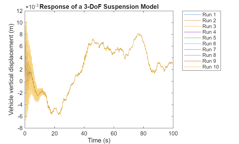
To see how varying the damping coefficient affects the vehicle dynamics, plot the vertical vehicle displacements.
Access the
SimulationOutputobject for each simulation. TheSimulationOutputobject contains a property for each type of logged data.Access the logged signal data using dot notation. Within each
SimulationOutputobject, signal logging data and metadata are grouped in aSimulink.SimulationData.Datasetobject with the default name oflogsout.Access the
vertical_dispsignal usingget.Access the
timeseriesobject that contains the time and signal data forvertical_dispusing theValuesproperty of thevertical_dispsignal.Plot the results for each simulation.
legend_labels = cell(1,numSims);
for idx = numSims:-1:1
    simOut = out(idx);
    sigLoggingData = simOut.logsout;
    sig = get(sigLoggingData,"vertical_disp");
    ts = sig.Values;

plot(ts);
    legend_labels{idx} = "Run "+num2str(idx);
    hold on
end

title("Response of a 3-DoF Suspension Model")
xlabel("Time (s)");
ylabel("Vehicle vertical displacement (m)");
legend(legend_labels,Location="NorthEastOutside");

Close MATLAB Workers
Close the parallel pool.
delete(gcp("nocreate"));Parallel pool using the 'Processes' profile is shutting down.
See Also
parsim | Simulink.SimulationInput | Simulink.Simulation.Variable