Frequency Response of Lowpass Chebyshev Filter
Use the Filter block to study the frequency response of a lowpass Chebyshev filter.
From the MATLAB® command prompt, open the model.
open_system('ex_simrf_filter_lowpass_cheby_resp')
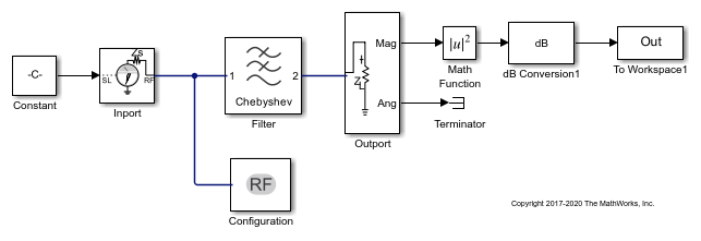
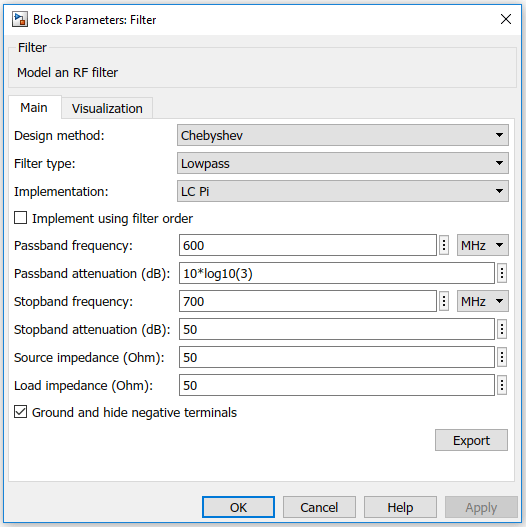
The Constant block sets the amplitude of the 201 carrier signals to ones (1, 201). The Inport block generates the 201 carrier frequencies for the mask value of logspace (7, 9, 201). Generate an 11th order lowpass LC Pi Chebyshev filter by setting appropriate block parameters in the Filter block.
The output signal from the Filter block is fed into the Outport block. The Outport block is configured to give both magnitude and angle of the signal. The angle output is terminated using the Terminator block. The magnitude output is squared and converted to dB using Math Function and dB Conversion blocks.
To run the model, select Simulation > Run. You can also use the following command:
sim('ex_simrf_filter_lowpass_cheby_resp')
The model creates an Out array in the MATLAB workspace. Since the simulation stop time is set to 0, the frequency response corresponds to the steady state solution.
To plot the frequency response, use the following commands in the MATLAB command window.
 figure
 freq = logspace(7,9,201);
 h = semilogx(freq, Out, '-gs', 'LineWidth',1, 'MarkerSize',3, 'MarkerFaceColor','r');
 xlabel('Frequency [Hz]');
 ylabel('Amplitude [dB]');
 title('Frequency Response of Lowpass Chebyshev Filter');
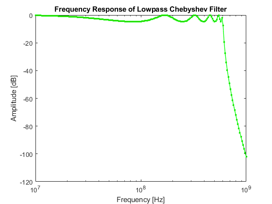
You can also use the Plot button in the Visualization tab of the Filter block parameters. Set the Frequency points to logspace (7, 9, 201) and X-axis scale to Logarithmic to achieve a similar plot.

See Also
Filter | <docid:simrf_ref#bvft10g-1> | <docid:simrf_ref#bvft_bs-1> | <docid:simrf_ref#bvflpaq>