M/M/1 Queuing System
Overview
An M/M/1 queue is a queuing system that has a Poisson arrival process, an exponential service time distribution, and one server. This example models an M/M/1 queuing system with a single traffic source and infinite storage capacity.
Queuing theory provides exact theoretical results for some performance measures of an M/M/1 queuing system. For example, for an arrival rate of  and a service rate of
  , the theoretical mean waiting time of an entity in the queue of an M/M/1 queuing system is given by:

where  is the mean total waiting time in a combined queue-server system and
  is the mean service time.
You can use this example to view and compare graphical plots of the theoretical mean wait times in the queue with the mean wait times measured during the simulation.
Explore the Model
Open the model.
modelname = "seMM1QueuingSys";
open_system(modelname);

The model has three main parts:
Entity Generation: Models entity generation that follows a Poisson arrival rate.
Entity Queuing: Models a queue of infinite storage capacity with a first-in, first-out (FIFO) policy.
Entity Service: Models a server with service times that follow an exponential distribution.
Entity Generation
This part of the model generates entities at a rate that follows a Poisson process. In a Poisson process, the times between entity generation are exponentially distributed. The entity intergeneration times are calculated using the value of arrival rate, .
The Knob block allows you to choose a value for the arrival rate by manually sliding the graphical knob around a circular, marked scale. For the purpose of this example, must be between 0.1 and 0.999. By default, the arrival rate is set to 0.5. A Simulink Function block, t = exponentialArrivalTime(), calculates entity intergeneration times that follow an exponential distribution given by the expression:
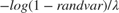
where randvar is the output of the Uniform Random Number block that represents random numbers uniformly distributed between 0 and 1, and is the arrival rate output by the Knob block.
The blocks calculating entity intergeneration times such as Math Function and Sum are grouped into a subsystem named Exponential Distribution.

The Entity Generator block generates entities at the Poisson arrival times using its intergeneration time action parameter. Open the Block Parameters dialog box of the Entity Generator block. The Generation Method parameter is set to Time-based and Time Source is set to MATLAB action. In the Intergeneration time action text box, variable dt that defines entity intergeneration times, is set to:

where exponentialArrivalTime() represents the output of the Simulink Function block with the same name.
Entity Queuing
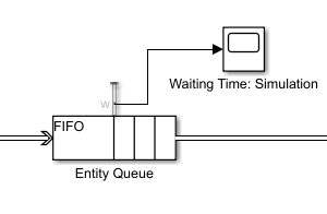
This part of the model queues entities after generation. Entities arriving to the system wait in the queue until the server is ready for processing. The queue has a first-in, first-out (FIFO) queuing policy and infinite storage capacity.
A Queue block is connected to the output of the Entity Generator block. Open the Block Parameters dialog box of the Entity Queue block. The Capacity parameter is set to inf and Queue type is set to FIFO. Go to the Statistics tab of the Block Parameters dialog box. Observe that the Average wait, w check box is selected.
A Scope block is connected to the average wait time output port, Port_w, of the Entity Queue block. It plots a graph of the average wait times of entities in the queue, as found during simulation.
Entity Service
This part of the model receives entities from the queue, and serves entities at service times that follow an exponential distribution. For the purpose of this example, the service rate is set to 1. The inverse of the service rate, which is the mean service time, is also 1.
An Entity Server block is connected to the output of the Entity Queue block. Open the Block Parameters dialog box of the Entity Server block. In the Service time action text box, variable dt that defines entity service times, is set to:

where mean is the mean service time which has a value of 1, and rand is a MATLAB function that returns a random number drawn from the uniform distribution in the interval (0,1).
After the service time elapses, entities leave the Entity Server block, and are terminated at an Entity Terminator block.
Simulate the Model
Simulate the model.
sim(modelname);
When you simulate the model, the Entity Generator block generates a new entity at the start time. When the entity departs the block, the Entity Generator block gets the intergeneration time variable, dt, to generate the next entity. This process then repeats.
Generated entities enter the Entity Queue block and wait until the Entity Server block is free to accept its next entity. The Entity Server is busy until the completion of service of its current entity, that is, until its service time has elapsed. The entity that completed service is terminated at the Entity Terminator block. An entity from the Entity Queue block that satisfies theFIFO policy takes up its place in the Entity Server. This cycle continues until the stop time of the simulation is reached.
Visualize the Output
These scopes are present in the model:
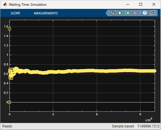
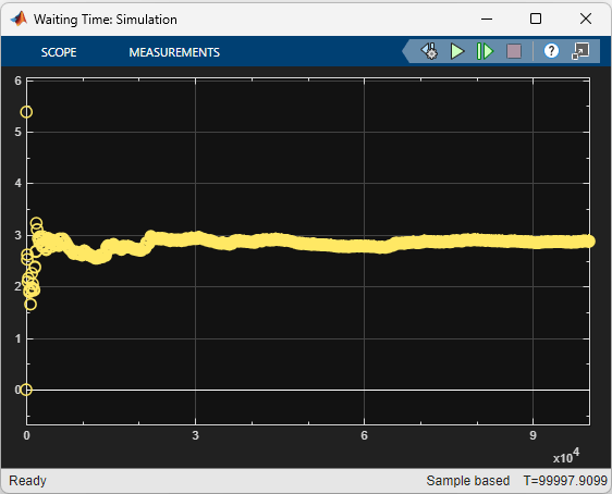
Waiting Time: Simulationplots the simulated values of mean waiting times in the queue. The simulated mean wait time is defined as the sum of the wait times of all entities that departed the block before the current time divided by their total number. It is plotted by the Scope block that is connected to the average wait time output port, Port_w, of the Entity Queue block.
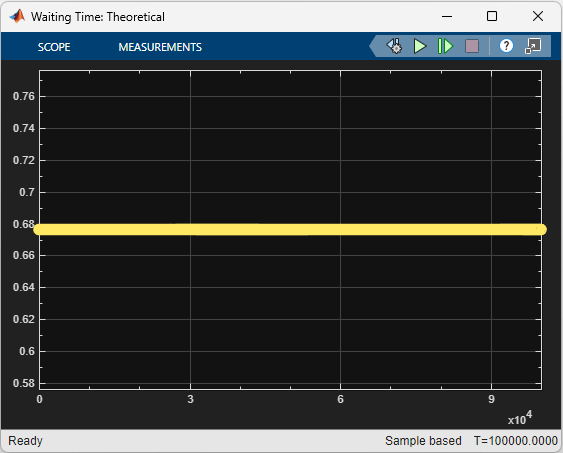
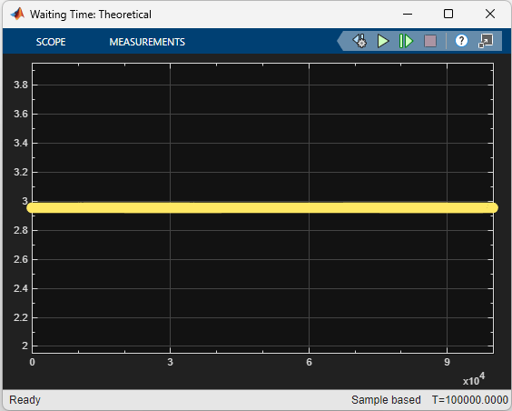
Waiting Time: Theoreticalplots the theoretical values of mean waiting times in the queue that is calculated by theCompute Theoretical Waiting Timesubsystem. This subsystem receives the arrival rate as input from the Knob block, and calculates the theoretical mean waiting time as: , where is the arrival rate, and is the service rate.
scopes = find_system(modelname, 'BlockType', 'Scope');
cellfun(@(x)open_system(x),scopes);


Move the Arrival Rate knob during the simulation and observe changes in the simulation results from the two Scope blocks.
This is a comparison of the simulated and theoretical mean waiting times, respectively, when the arrival rate is set to 0.4.
This is a comparison of the simulated and theoretical mean waiting times, respectively, when the arrival rate is set to 0.74.
References
Kleinrock, Leonard. Queueing Systems, Volume I: Theory. New York: Wiley, 1975.
See Also
Entity Generator | Entity Server | Queue | Entity Terminator