Main Content

Zero-Pole Analysis

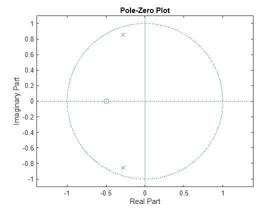
The zplane function plots poles and zeros of a linear system. For example, a simple filter with a zero at -1/2 and a complex pole pair at 0.9e-j2π0.3 and 0.9ej2π0.3 is

zer = -0.5; 
pol = 0.9*exp(j*2*pi*[-0.3 0.3]');

To view the pole-zero plot for this filter you can use zplane. Supply column vector arguments when the system is in pole-zero form.

zplane(zer,pol)

Figure contains an axes object. The axes object with title Pole-Zero Plot, xlabel Real Part, ylabel Imaginary Part contains 3 objects of type line. One or more of the lines displays its values using only markers

For access to additional tools, use fvtool. First convert the poles and zeros to transfer function form, then call fvtool.

[b,a] = zp2tf(zer,pol,1);
fvtool(b,a)

Figure Figure 1: Magnitude Response (dB) contains an axes object. The axes object with title Magnitude Response (dB), xlabel Normalized Frequency ( times pi blank rad/sample), ylabel Magnitude (dB) contains an object of type line.

Click the Pole/Zero Plot toolbar button, select Analysis > Pole/Zero Plot from the menu, or type the following code to see the plot.

fvtool(b,a,'Analysis','polezero')

Figure Figure 2: Pole-Zero Plot contains an axes object. The axes object with title Pole-Zero Plot, xlabel Real Part, ylabel Imaginary Part contains 3 objects of type line. One or more of the lines displays its values using only markers

To use zplane for a system in transfer function form, supply row vector arguments. In this case, zplane finds the roots of the numerator and denominator using the roots function and plots the resulting zeros and poles.

zplane(b,a)

Figure contains an axes object. The axes object with title Pole-Zero Plot, xlabel Real Part, ylabel Imaginary Part contains 3 objects of type line. One or more of the lines displays its values using only markers

See Discrete-Time System Models for details on zero-pole and transfer function representation of systems.

See Also

| |