Common Periodic Waveforms

Signal Processing Toolbox™ provides functions for generating widely used periodic waveforms.

• sawtooth generates a sawtooth wave with peaks at $$\pm 1$$ and a period of $$2\pi$$. An optional width parameter specifies a fractional multiple of $$2\pi$$ at which the signal maximum occurs.

• square generates a square wave with a period of $$2\pi$$. An optional parameter specifies the duty cycle, the percent of the period for which the signal is positive.

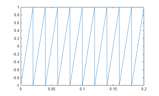
Generate 1.5 seconds of a 50 Hz sawtooth wave with a sample rate of 10 kHz. Plot 0.2 seconds of the generated waveform.

fs = 10e3;
t = 0:1/fs:1.5;
x = sawtooth(2*pi*50*t);

plot(t,x)
axis([0 0.2 -1 1])

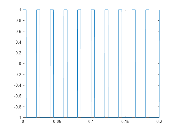
Generate 1.5 seconds of a 50 Hz square wave with a sample rate of 10 kHz. Specify a duty cycle of 25%. Plot 0.2 seconds of the generated waveform.

fs = 10e3;
t = 0:1/fs:1.5;
x = square(2*pi*50*t,25);

plot(t,x)
axis([0 0.2 -1 1])

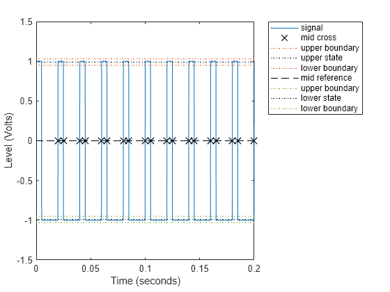
Use the dutycycle function to verify that the duty cycle of the square wave is the specified value. Use the function with no output arguments to plot the waveform, the location of the mid-reference level instants, the associated reference levels, the state levels, and the associated lower and upper state boundaries.

dc = dutycycle(x,fs);
dc = dc(1)

dc = 
0.2500

dutycycle(x,fs);
xlim([0 0.2])