Analysis Flow in Serial Link Design
The Serial Link Designer app uses an iterative and sequential process to narrow down a large solution space and arrive at an optimal solution. This diagram explains the workflow followed by the app.
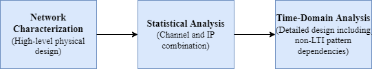
This flow is supported by both pre-layout (solution space exploration and progressive analysis) and post-layout (single or multi-board extraction and analysis).
Network Characterization
The network characterization section in the workflow determines if the high-level physical design of the link meets the design requirements. The Serial Link Designer app automatically detects the modeling techniques used in designing the transmitter and the receiver,and then determines the analysis workflow based on the models used.
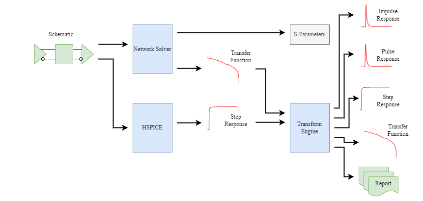
You can perform network characterization in the Serial Link Designer in two ways:
Using the Serial Link Designer network solver
Using SPICE transient simulation to get the step response
Network Characterization Results
| Result | Description |
|---|---|
| Impulse Response | Impulse response is the response of the channel to an extremely short pulse with unit area. In sampled data analysis, the width of the pulse is one sample, and the amplitude is one sample over the sample interval. The impulse response measurement is a mathematical construct and is not realizable in practice. The impulse response outputs from the Serial Link Designer app help determine the path delay. They also indicate the extent of the distortion due to reflections in the transmission path. The impulse response shows the high frequency response more clearly than pulse response or step response. |
| Pulse Response | The pulse response is the response of the path to a pulse which is one data symbol wide, and has an amplitude equal to the difference between a logical zero and a logical one. Pulse responses are particularly useful for understanding the effects of equalization. The sampling time after clock recovery is typically very near the peak of the pulse response. As a result, the most critical intersymbol interference occurs an integer number of bit times from the peak of the pulse response.
|
| Step Response | The Serial Link Designer calculates the step response assuming the 0-100% rise time of the step is one sample interval, and the step is from a logical zero to a logical one. Since a step response is physically realizable, it is useful for comparing results from the app with results from other simulators such as the SPICE simulator. It is also useful for comparing the app results directly with measured time domain reflection (TDR) and time domain transmission (TDT) responses For small impedance discontinuities, the TDR response is approximately a plot of the transmission line impedance as a function of distance. For this reason, the Serial Link Designer app produces a step response for the output of each driver, even though it does not produce a corresponding impulse response, pulse response, or transfer function for these circuit nodes. In the Signal Integrity Viewer app, the TDR step responses are indicated as V(Bxxx to TDR) to distinguish them from the other step responses. |
| Transfer Function | The Serial Link Designer app outputs transfer functions of the real and imaginary parts as a function of frequency. In the Signal Integrity Viewer app, this data is then combined to show magnitude (dB or linear), phase, and polar plots in addition to real and imaginary parts. Since the transfer functions include the drivers and receive amplifiers, they can exhibit gain, especially at low frequencies. |
| Output S-Parameters | The Serial Link Designer app outputs S-parameters for the channel in a fully-compliant Touchstone file. Each driver and receiver pin is a separate single ended port, and the file contains a comment line listing the node names of the ports in order. The S-parameters are output from DC to a frequency set by the Max Output Frequency (default is 10GHz) parameter in steps set by the parameter S-Parameter Frequency Step (default is 50MHz) parameter. |
For more information, see Network Characterization Results.
Statistical Analysis
Statistical Analysis uses the network characterization results and the IBIS-AMI models to derive the statistical eye, BER estimate, and other data. The analysis assumes LTI (linear time invariant) channel and LTI equalization.
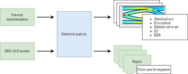
The Transmit and Receive equalization is applied by the IBIS-AMI models. The IBIS-AMI Init function takes an impulse response and returns that impulse response convolved with the equalization impulse response.
To estimate the BER, you must obtain the clock PDF. If the IBIS-AMI model does not return a clock PDF, then an internal CDR will produce its own clock PDF.
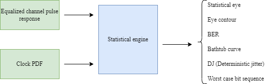
The statistical engine takes the equalized channel pulse response and the clock PDF and generates the outputs.
There are simulation parameters that affect the statistical analysis results. For more information on the simulation parameters, see Simulation Parameters Used in Serial Link Design.
Statistical Analysis Results
| Result | Description |
|---|---|
| Statistical Eye | The statistical eye is a false color plot of the probability at each voltage as a function of time relative to the bit sampling time. The underlying assumption is that all messages of a given length (typically 64 bits or more) are equally likely, and the probabilities are therefore the average over all possible combinations of intersymbol interference for that message length. In the Serial Link Designer app, the statistical eye also includes the effects of crosstalk. The statistical eye is centered by assuming that the clock recovery loop will choose the median threshold crossing time as the edge of the eye, and position the data sampling time one-half a bit time from the edge of the eye. This behavior can be obtained from an ideal digital clock recovery loop. The viewer displays the statistical eye by color coding the probabilities in rainbow order with red being the highest probability and blue the lowest probability. |
| Bathtub Curve Set | The bathtub curve set consists of three curves:
|
| DJ (Deterministic jitter) | The DJ curve is a histogram of the threshold crossing times for the data. It is used primarily to help better understand the DJ peak and standard deviation entries. |
| Contours | The eye contours are plots of the amplitude associated with fixed probabilities as a function of sampling time. They indicate the shape of the inner and outer boundaries of the eye diagram for a number of different probabilities. The contour curve set also includes the peak distortion analysis (PDA) curves. These contours indicate the absolute inner and outer boundaries of the statistical eye. |
For more information, see Statistical Analysis Results.
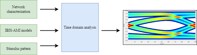
Time-Domain Analysis
Time-domain analysis uses the network characterization results, IBIS-AMI models, and a bit sequence to derive the output waveform, BER estimate, and other data.
To estimate the BER, you must obtain the clock PDF from one of the two sources:
CDR in the Receiver IBIS-AMI model.
Internal CDR built into Signal Integrity Toolbox™.
There are simulation parameters affect the time domain analysis results. For more information on the simulation parameters, see Simulation Parameters Used in Serial Link Design.
Time Domain Analysis Results
| Result | Description |
|---|---|
| Persistent Eye | The persistent eye is the amplitude statistics accumulated from a specific time domain waveform. It is accumulated when you trigger the use of an ideal recovered clock, in exactly the same way that an eye diagram is accumulated in a modern digital sampling scope. In Clock Mode Normal, the data is clocked using a clock recovery loop that is internal to the analysis probe of the app. This clock recovery loop is an analog Hogg and Chu style delay locked loop. For 6.25 Gb/s data, the pattern dependent jitter from this clock recovery loop is slightly less than 1 pS rms. Since it is an analog rather than a digital clock recovery loop, it locks to the mean data transition time rather than the median. If the Receiver IBIS-AMI Model contains a CDR, the resulting clock PDF will represent this CDR, and not the internal clock recovery loop. In Clock Mode Clocked the actual recovered clock ticks are used to sample the data if the clock ticks are available from the receiver model. For more information, see Clock Modes. The appearance and meaning of the persistent eye is very similar to that of a statistical eye except that it represents the density accumulated from a specific time domain waveform rather than the probability calculated for a population of messages. |
| Bathtub Curve Set | The bathtub curve set for a time domain simulation is derived from the persistent eye. Depending on the clock mode, the clock PDF can be accumulated from the clock ticks produced by an IBIS-AMI receiver model rather than the RJ and SJ specified for the receiver. |
| DJ (Deterministic jitter) | The DJ curve is a histogram of the threshold crossing times for the data. The DJ for a time-domain simulation is derived from the persistent eye. |
| Contours | The eye contours are plots of the amplitude associated with fixed probabilities as a function of sampling time. They indicate the shape of the inner and outer boundaries of the eye diagram for a number of different probabilities. The contours for a time-domain simulation are derived from the persistent eye. Since the persistent eye is necessarily derived from a relatively small sample (typically one million to ten million bits), the contours for lower probabilities are not resolvable. No attempt is made to separate these curves through any method such as statistical extrapolation. Statistical extrapolation is available as an option in the simulation parameters. |
For more information, see Time Domain Analysis Results.
Pre-Layout Analysis
The schematic in the network characterization diagram represents an uncoupled net or a coupled net. Uncoupled nets can be thought of as net classes. The Serial Link Designer app stores this information as a transfer net, which is used as the underlying data structure for all analyses. You can reuse the transfer net data can be re-used between pre- and post-layout analysis and between designs. Reusing analysis setups with common interfaces across multiple designs can save significant time and resources when performing signal integrity, timing, and crosstalk analysis.
The pre-layout analysis is an interface-centric iterative process used to generate design guidelines for your board layouts, package layouts, connectors, and cabling. For more information, see Pre-Layout Analysis of Serial Link.
Post-Layout Analysis
The post-layout process supports the PCB analysis of single-board and multi-board designs. You can analyze the connectivity through packages, connectors, and cabling. For more information, see Post-Layout Verification of Serial Link.