Level Separation Mismatch Ratio (RLM) using IBIS-AMI

This example shows how to add Transmitter Level Mismatch (RLM) to a transmitter (Tx) and how to calculate the resulting level separation mismatch ratio at the receiver (Rx) with IBIS-AMI models.

Background

Level Separation Mismatch Ratio, commonly known as $$R_{LM}$$, is a measure of the irregularity of the various eye openings in a PAMn signal. It is calculated by dividing the minimum eye opening by the average eye opening of all the PAMn eyes, where the eye openings are determined by the mean value of each symbol voltage. An $$R_{LM}$$ of 1 means that the system is perfectly linear. This example uses SerDes Toolbox™ to show how to inject $$R_{LM}$$ into the stimulus pattern at the input to a Tx IBIS-AMI model, and how to measure the final $$R_{LM}$$ at the output of a Rx IBIS-AMI model.

Since RLM models non-LTI behavior in the Transmitter, $$R_{LM}$$ is a GetWave only feature.

Model Setup in SerDes Designer App

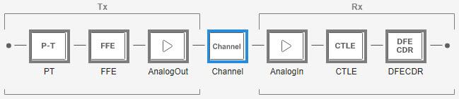
The first part of this example sets up some typical Tx and Rx equalization blocks using the SerDes Designer app. Launch the app with the following command:

serdesDesigner

Configuration Setup

Begin by setting the following values in the Configuration tab in the app toolstrip:

• Set the Symbol Time to 200ps (5.0GHz).

• Set the Modulation to PAM3.

• Set the Signaling to Single-ended.

Tx Model Setup

Add a Pass-Through block and a FFE block to the Tx, keeping the default settings. Keep the default settings for the AnalogOut model as well. The Pass-Through block is used to inject the $$R_{LM}$$ at the input to the Tx, while the FFE is simply a standard Tx equalization block.

Analog Channel Setup

• Verify the Channel loss is set to 8 dB and the Single-ended impedance is set to 50 ohms.

• Set the Target Frequency to 2.5 GHz, which is the Nyquist frequency for 5.0 GHz.

Rx Model Setup

Keep the default settings for the AnalogIn model, then add a CTLE and a DFECDR block to the Rx. Keep the default settings for these blocks.

The final SerDes system should look like this:

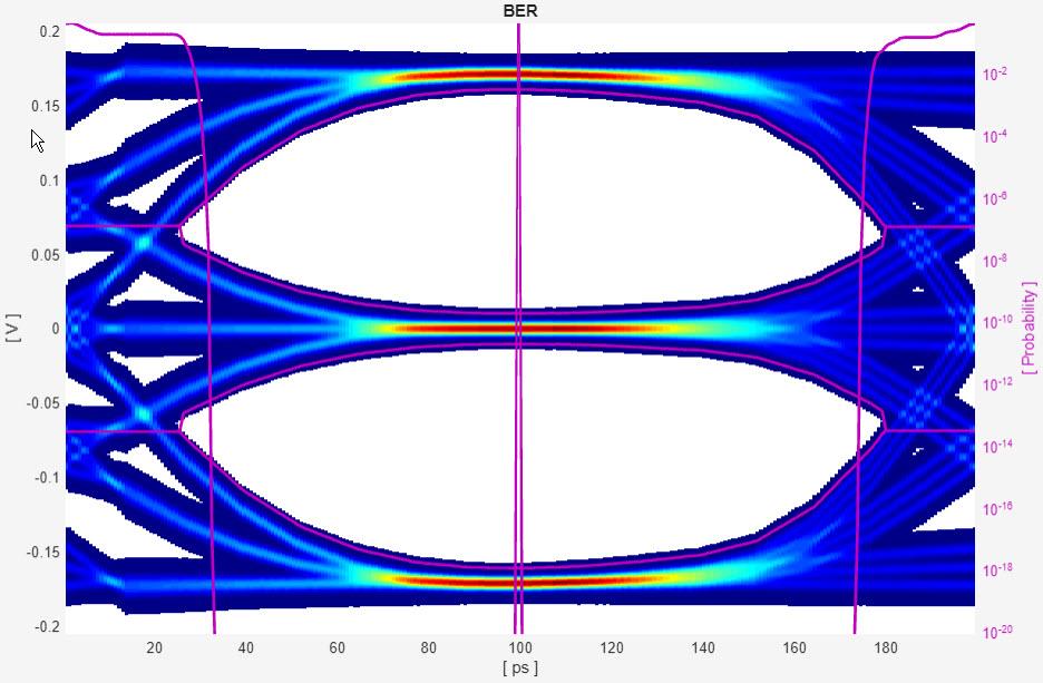
Plot Statistical Results

Use the SerDes Designer Add Plots button to visualize the results of the setup. Add the BER plot from Add Plots and observe the result:

Export SerDes System to Simulink

Click Save and then click on the Export button to export the configuration to Simulink®, where you will add support for $$R_{LM}$$ to the Tx and Rx blocks.

Model Setup in Simulink

The second part of this example takes the SerDes system exported by the SerDes Designer app and customizes it in Simulink.

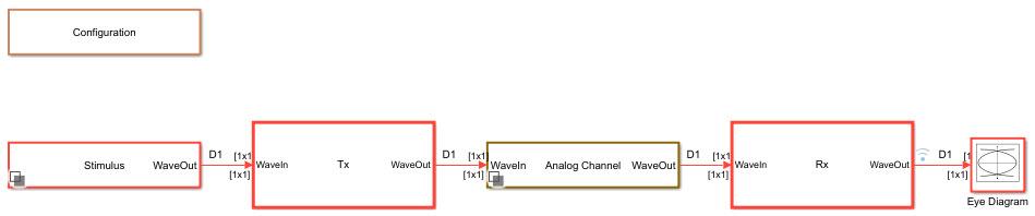
Review Simulink Model Setup

This Simulink SerDes system contains the standard configuration: Stimulus, Configuration, Analog Channel, Tx and Rx blocks, with all values carried over from the SerDes Designer app. Review each of these blocks to verify the setup is as expected.

Add RLM Generation to the Tx Model

Look under the Tx subsystem, then rename the Pass-Through block from PT to RLM_Injection to better describe its operation.

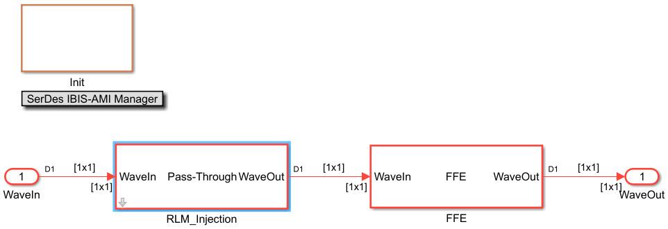
Edit the Pass-Through Block

Next, look under the mask of the RLM_Injection block:

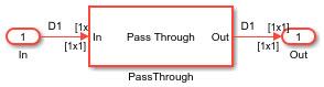
Delete the Pass-Through block and add a MATLAB Function block to the canvas. Edit the MATLAB Function block and replace the entire contents with the following code:

function stimOut = RLM_Injection(stimIn, sign, RLM, Modulation)
% stimOut    Add Transmitter Level MisMatch to incoming stimulus signal.
%            Uses a saturating non-linearity to shift a single symbol
%             voltage on the incoming stimulus waveform.
%            Supports PAMn for N > 2
%            Not valid for NRZ
%
% stimIn     Stimulus input
% sign       Sign of RLM to be added: 1 (positive) or -1 (negative)
% RLM        Ratio of Level MisMatch (RLM) should be between 0.5 and 1.0
%             Only the upper eye is modified by varying the N-1 symbol voltage.
% Modulation Current modulation being used. Passed in via Data Scope = Parameter.
% stimOut    Stimulus output with RLM added.

% Copyright 2023 The MathWorks, Inc.

% Skip entire function if NRZ
if Modulation == 2
    stimOut = stimIn;
    return
end

persistent vinvout

if isempty(vinvout)
    % Do not allow RLM smaller than 0.5
    if RLM < 0.5
        RLM = 0.5;
    end

    % Determine amount to shift incoming stimulus waveform
    bias = sign*(1-abs(RLM))/(Modulation - 1);

    Vswing = 0.5;       %% +/- Input signal swing
    Vstep  = 0.005;     %% Minimum voltage step in Vin/Vout array

    % Voltage range to apply bias to
    limit = 0.5/(Modulation - 1);
    % Center of Symbol voltage to be shifted
    Vcent = abs((Vswing * 2)/(Modulation - 1) - Vswing);
  
    % Define incoming voltage points
    vin1 = -Vswing * 2;
    vin2 = -Vswing;
    vin3 =  Vcent - limit/2 - Vstep;
    vin4 =  Vcent - limit/2;
    vin5 =  Vcent;
    vin6 =  Vcent + limit/2;
    vin7 =  Vcent + limit/2 + Vstep + bias;
    vin8 =  Vswing;
    vin9 =  Vswing * 2;
        
    % Define outgoing voltage points
    vout1 = vin1;
    vout2 = vin2;
    vout3 = vin3;
    vout4 = vin4 + bias;
    vout5 = vin5 + bias;
    vout6 = vin6 + bias;
    vout7 = vin7;
    vout8 = vin8;
    vout9 = vin9;

    vinvout = [vin1 vout1; vin2 vout2; vin3 vout3; vin4 vout4; vin5 vout5; vin6 vout6; vin7 vout7; vin8 vout8; vin9 vout9];

end

%% Apply memory-less non-linearity from serdes.SaturatingAmplifier
vin  = vinvout(:,1);
vout = vinvout(:,2);

% Perform lookup operation. Inspired by Bentley's binary search in "Programming Pearls".
% Initialize Search Index
lo = 1;
hi = length(vin);

if stimIn <= vin(lo)
    stimOut = vout(lo);
elseif stimIn > vin(hi)
    stimOut = vout(hi);
else
    while hi > lo+1
        mid = round((hi+lo)/2);
        if stimIn <= vin(mid)
            hi = mid;
        else
            lo = mid;
        end
    end
    % Linear interpolation: No need to protect against
    %  divide by zero since it is guaranteed that hi~=lo
    stimOut = (vout(hi)*(stimIn-vin(lo)) + ...
        vout(lo)*(vin(hi)-stimIn) )/...
        (vin(hi) - vin(lo) );
end

Note: In the function signature for the RLM_Injection MATLAB function, you must change the Data Scope for the parameter "Modulation" from Input to Parameter.

Rename the MATLAB function block to RLM_Injection so that the resulting waveform names in the Simulation Data Inspector becomes more intuitive.

Add Tx AMI Parameters

Open the SerDes IBIS-AMI Manager and select the AMI-Tx tab. Highlight the RLM_Injection block and add two new AMI Parameters:

Parameter name: RLM_sign

• Usage: In

• Type: Integer

• Format: List

• Default: 1

• List values: [1 -1]

• List-Tip values: ["Positive" "Negative"]

• Description: RLM bias sign. +1 adds a positive bias. -1 adds a negative bias.

• Verify the Current value is: Positive

Parameter name: RLM_input

• Usage: In

• Type: Float

• Format: Range

• Typ: 1

• Min: 0.5

• Max: 1

• Description: Target Transmitter Level Mismatch (RLM) value. RLM = 1 means no distortion in transmitted symbol voltages.

• Current value: 1

Connect Everything Up

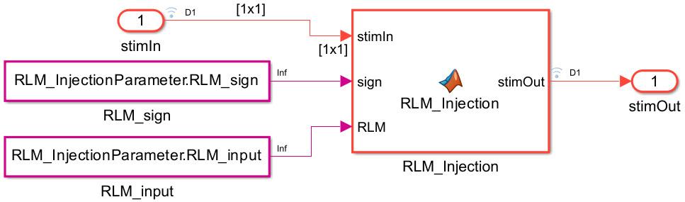
Wire up the input and output ports, along with the two new AMI parameters to the RLM_Injection MATLAB function block. You can also turn logging on for the stimIn and stimOut nodes to visually verify the operation of the $$R_{LM}$$ Injection.

The final pass-through block should look like this:

Add RLM Calculation to the Rx Model

Push into the Rx subsystem, then look under the mask of the DFECDR block.

Edit the DFECDR Block

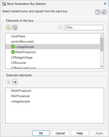
Edit the Bus Selector and add the element voltageSample to the output:

Add a MATLAB Function block to the canvas. Edit the MATLAB Function block and replace the entire contents with the following code:

function RLM_Out = RLM_Calculation(PAMThreshold, voltageSample, ignoreBits, rlmWindowSize, Modulation, SymbolTime, SampleInterval)
% RLM_Calculation    Calculates the Ratio of Level MisMatch (RLM) value, also known as
%                     Level Separation MisMatch Ratio.
%                    Supports PAMn for N > 2
%                    Not valid for NRZ
%
% PAMThreshold     Vector of PAM Thresholds for each eye in the PAMn modulation. Generated by CDR.
% voltageSample    Voltage observed from the dtaa signal at the Clock Time. Generated by the CDR.
% ignoreBits       Integer number of bits to ignore before starting the RLM Calculation. Value
%                   passed in via AMI Parameter.
% rlmWindowSize    Integer number of bits to include in each RLM calculation. Value passed in
%                   via AMI Parameter.
% Modulation       Current Modulation being used. Passed in via Data Scope = Parameter.
% SymbolTime       Current simulation Symbol Time. Passed in via Data Scope = Parameter.
% SampleInterval   Current simulation Sample Interval. Passed in via Data Scope = Parameter.
% RLM_Out          Calculated RLM value.
%
% Copyright 2023 The MathWorks, Inc.

% Skip entire function if NRZ
if Modulation == 2
    RLM_Out = 1;
    return
end

% Set up persistent variables to be available between time steps
persistent vsArray sampCount rlmWinCount tempRLM_Out uiCount sampBit delta

if isempty(sampBit)
    sampBit = round(SymbolTime/SampleInterval);
    sampCount = int32(0);     %% Total elapsed samples
    rlmWinCount = int32(0);   %% Window size counter
    uiCount = int32(0);       %% Total UI counter
    delta = zeros(1, Modulation-1);
    vsArray = 0;
    tempRLM_Out = 1;
end

% Initialize output to previous value
RLM_Out = tempRLM_Out;

% Track number of elapsed samples
sampCount = sampCount + 1;

% Accumulate voltage samples every UI
if mod(sampCount,sampBit) == 0
    vsArray = [vsArray voltageSample];
    rlmWinCount = rlmWinCount + 1;
    uiCount = uiCount + 1;
end

% Calculate new RLM value every rlmWindowSize
if (rlmWinCount >= rlmWindowSize && uiCount > ignoreBits)
 
    minV = min(vsArray);
    maxV = max(vsArray);   
    Vmean = zeros(1, Modulation);

    % Calculate lowest mean value (V0)
    Vzero = vsArray((vsArray >= minV) & (vsArray < PAMThreshold(1)));
    Vmean(1) = mean(Vzero);
    
    % Calculate middle mean value(s)
    for jj = 1:Modulation-2
        Vnext = vsArray((vsArray > PAMThreshold(jj)) & (vsArray < PAMThreshold(jj+1)));
        Vmean(jj+1) = mean(Vnext);
    end
    
    % Calculate highest mean value
    Vlast = vsArray((vsArray >= PAMThreshold(Modulation-1)) & (vsArray <= maxV));
    Vmean(Modulation) = mean(Vlast);
    
    % Calculate final RLM value
    for kk = Modulation:-1:2
        delta(kk-1) = Vmean(kk) - Vmean(kk-1);
    end
    num = min(delta);
    den = (Vmean(Modulation)-Vmean(1)) / (Modulation-1);
    RLM_Out = num/den;

    % Reset for next rlm Window
    vsArray = 0;
    rlmWinCount = int32(0);

end

% Save result for next iteration
tempRLM_Out = RLM_Out;

Note: In the function signature for the RLM_Calculation MATLAB function, you must change the Data Scope for the parameters "Modulation", "SymbolTime" and "SampleInterval" from Input to Parameter.

Rename the MATLAB function block to RLM_Calculation so that the resulting waveform names in the Simulation Data Inspector become more intuitive.

Add Rx AMI Parameters

Open the SerDes IBIS-AMI Manager and select the AMI-Rx tab. Highlight the DFECDR block and add three new AMI Parameters:

Parameter name: RLM_ignoreBits

• Usage: In

• Type: Integer

• Format: Range

• Typ: 1000

• Min: 10

• Max: 1000000

• Description: Number of bits to ignore at the beginning of the simulation when calculating the RLM value (Time Domain only).

• Current value: 1000

Parameter name: RLM_windowSize

• Usage: In

• Type: Integer

• Format: Range

• Typ: 1000

• Min: 50

• Max: 100000

• Description: Number of bits to use in RLM calculation.

• Current value: 1000

Parameter name: RLM_Value

• Usage: Out

• Type: Float

• Format: Value

• Description: Value of the Level Separation Mis-Match Ratio.

• Current value: 1

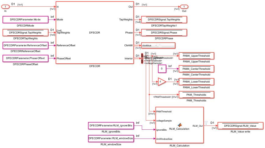
Connect Everything Up

Wire up the two new AMI Input parameters, the new AMI Output parameter, and the two Bus Selector signals PAMThreshold and voltageSample to the MATLAB Function block RLM_Calculation. You can also turn logging on for the RLM_Out node to visually verify the operation of the RLM Calculation.

The final DFECDR block should look like this:

Test the Simulink Model Operation

The full Simulink model is ready to run. It is recommended to set the Rx Bits to ignore to at least 15000 in the IBIS-AMI Manager to allow time for the DFE and CTLE to settle. Run the simulation.

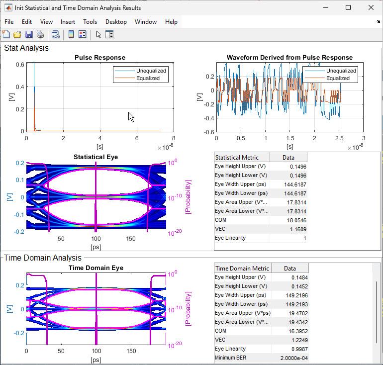
With the Tx RLM_input set to 1, the Init Statistical and Time Domain Analysis Results dialog should look similar to this:

Tx Model Testing

Set the Tx RLM_input to 0.8 and the RLM_sign to Positive in the IBIS-AMI Manager, then re-run the model:

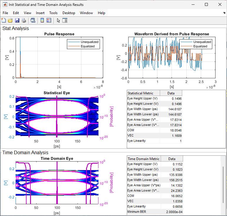
Note how the Time Domain upper eye height has closed down while the lower eye height has opened up. Also notice that since RLM is only applied to the GetWave portion of the model, the Statistical results remain unchanged.

Now leave the Tx RLM_input at 0.8 but change the RLM_sign to Negative in the IBIS-AMI Manager, then re-run the model:

This time, the upper eye height has opened up and the lower eye height has closed down.

To verify that the RLM_Injection block is operating correctly, use the Simulation Data Inspector to plot the output of the RLM_Injection pass-through block for the last two simulations:

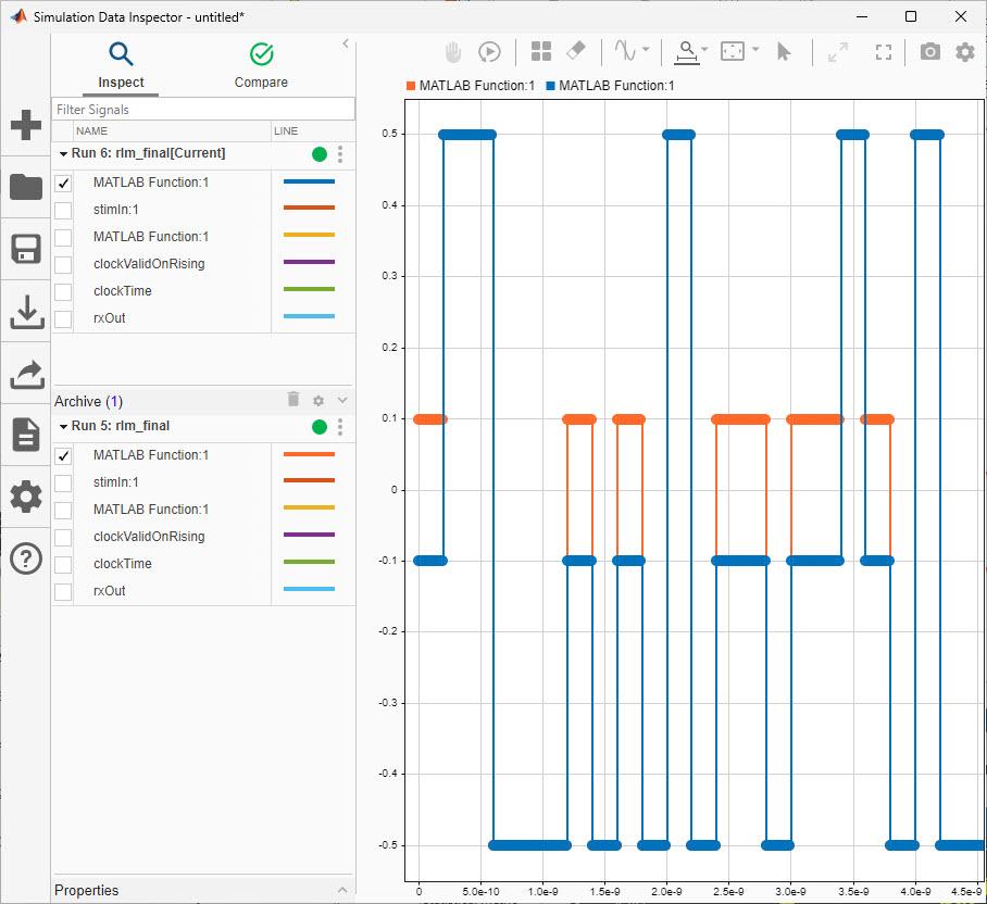
The red waveform is the output when RLM_sign was Positive, and the blue waveform is the output when RLM_sign was Negative. In both cases the RLM_input was set to 0.8. Note that the high (+0.5V) and low (-0.5V) symbol voltages are unchanged.

Repeat the last two simulations using PAM4 modulation and see how the eyes change. Note that only the upper PAMn eye is modified by RLM.

How Does the RLM Injection Work

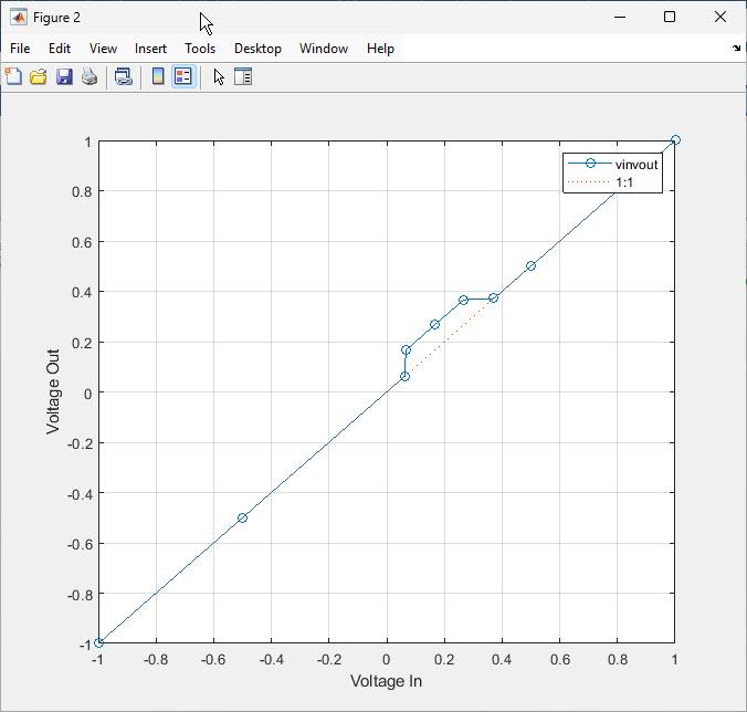
PAM3 has symbol voltages of -0.5, 0 and +0.5V, while PAM4 has symbol voltages of -0.5, -0.1667, +0.1667 and +0.5. The $$R_{LM}$$ injection algorithm works by using a saturating nonlinearity to shift the N-1 symbol voltage while leaving the remaining symbol voltages alone. In order to account for any jitter or noise added to the incoming stimulus, a range of voltages around the N-1 symbol voltage (0.0V for PAM3 or 0.1667V for PAM4) are shifted.

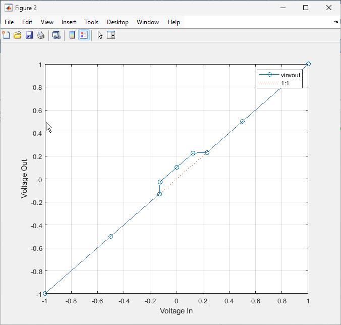
The Vin/Vout saturation curve for PAM3 with RLM_input set to 0.8 and RLM_sign Positive looks like the following:

The Vin/Vout saturation curve for PAM4 with RLM_input set to 0.8 and RLM_sign Positive looks like the following:

Limitations to Tx RLM Injection

While $$R_{LM}$$ Injection will work for any PAMn modulation, it only operates on the N-1 symbol threshold so only the top-most eye can be made larger or smaller.

Rx Model Testing

Use the Configuration block to set the Modulation to PAM3, then verify that the Tx RLM_input is set to 0.8 and the RLM_sign is Positive in the IBIS-AMI Manager. Run the simulation, then plot the signal RLM_Calculation:1 in the Simulation Data Inspector. If this signal is not available, make sure that you have enabled logging on the output of the MATLAB Function block in the DFECDR and that the MATLAB Function block has been named RLM_Calculation. The plot should look similar to this:

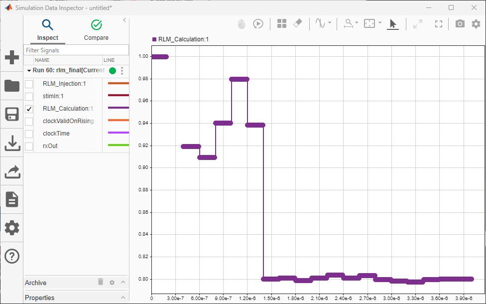
Note that the RLM calculation bounces around quite a bit as the CTLE and DFE taps adapt before finally settling at ~0.8 as expected.

Now, change the AMI Parameter RLM_ignoreBits from 1000 to 10000 and re-run the simulation:

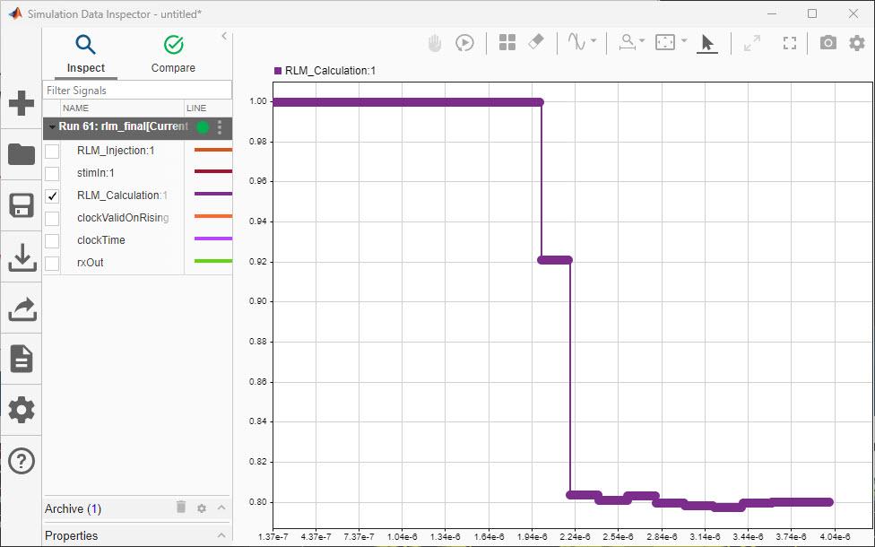
Note that the RLM calculation stays at the default value of 1.0 until after 10,000 bits (half the simulation time) before quickly settling to ~0.8.

Finally, set the AMI Parameter RLM_ignoreBits back to 1000, and set AMI_windowSize to 5000 and re-run the simulation:

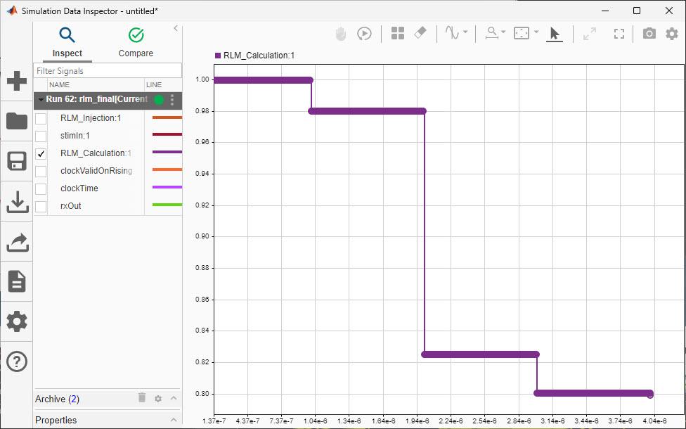
Note that while the $$R_{LM}$$ calculation is adapting much more slowly, it does not jump around nearly as much when using the larger window size to make each calculation.

How does the RLM Calculation work

The RLM calculation works by starting with each PAM threshold value, them moving up and down to find the limits of each symbol voltage. The average value V of each symbol voltage is used to calculate the final RLM value using the equation:

$$\mathit{R}\mathrm{LM}=\frac{\min \left({\mathit{V}}_{\mathit{N}}-{\mathit{V}}_{\mathit{N}-1},{\mathit{V}}_{\mathit{N}-1}-{\mathit{V}}_{\mathit{N}-2},...{\mathit{V}}_2-{\mathit{V}}_{\mathit{1}}\right)}{\left({\mathit{V}}_{\mathit{N}}-{\mathit{V}}_1\right)/\mathit{N}-1}$$

No calculations are performed until after RLM_ignoreBits has elapsed, and the number of UI contained in each RLM calculation is determined by the value of RLM_windowSize.

Generate IBIS-AMI Models

The final part of this example takes the customized Simulink model and generates IBIS-AMI compliant model executables, IBIS and AMI files for the RLM-enabled transmitter and receiver.

Export Models

Open the SerDes IBIS-AMI Manager and select the Export tab. On the Export tab:

• Update the Tx model name to rlm_tx

• Update the Rx model name to rlm_rx.

• Note that the Tx and Rx corner percentage is set to 10. This will scale the min/max analog model corner values by +/-10%.

• Verify that Dual model is selected for both the Tx and Rx AMI Model Settings. This will create a model executable that supports both statistical (Init) and time domain (GetWave) analysis.

• Set the Rx model Bits to ignore value to 1000 to allow enough time for the external clock waveform to settle during time domain simulations.

• Set Models to export to Both Tx and Rx.

• Set the IBIS file name to be rlm_models.ibs

• Press the Export button to generate models in the Target directory.

Test Generated IBIS-AMI Model Executables

The $$R_{LM}$$ capable IBIS-AMI models are now complete and ready to be tested in any industry standard AMI model simulator such as Signal Integrity Toolbox.

References

IBIS-AMI Specification