Generate HDL for Dual-Summing-Node DFE

This example shows how to design a bit-accurate decision feedback equalizer (DFE) adaptation engine for an architecturally representative 100-Gb/s dual-summing-node-DFE PAM4 SerDes receiver model using blocks from the SerDes Toolbox™. This bit-accurate DFE adaptation engine generates synthesizable RTL code that is suitable for implementation in an ASIC or an FPGA. The implementation-representative datapath in the DFE model enables the adaptation engine to reflect key design aspects: PAM4 threshold recovery, DFE tap weight adjustment, and clock phase sensitivity.

The example includes these sections:

1. Steps to advance the adaptation engine from an abstract, system-level Simulink® model to a bit-accurate, RTL-ready Simulink model.

2. Automated conversion of the adaptation engine from the bit-accurate Simulink model to synthesizable RTL code using HDL Coder™.

3. Validation of the adaptation engine design by comparing test-vectors between the RTL code simulated in Verilog and the bit-accurate model simulated in Simulink.

Example Overview

Historically, SerDes designs used a single-summing-node DFE topology. Due to increasing SerDes data rates, the DFE timing constraints become tighter and the design margins shrink, requiring alternative DFE topologies. One such topology is the dual-summing-node DFE. This DFE uses two summing nodes, rather than one: each summing node equalizes every other incoming symbol at half the speed to relax timing constraints and to reduce clock rates at the cost of increased circuit complexity and area [1]. This example uses an architecturally representative dual-summing-node-DFE PAM4 receiver model to illustrate a methodology for designing realistic adaptation engines ready for hardware implementation. At the same time, the model refines the representation of an IBIS-AMI model.

Model Overview

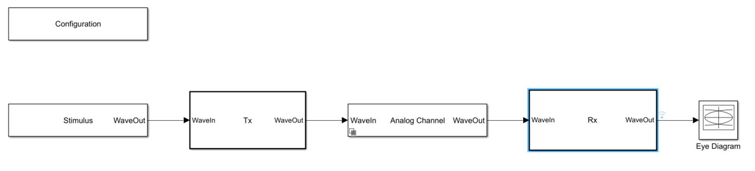
To access the dual-summing node DFE Simulink model, DualSummingNodeSerdes.slx, open the project provided with this example. This SerDes model is the starting point for this example and matches the model found in Architectural 100G Dual-Summing-Node-DFE PAM4 SerDes Receiver Model.

openProject('dual_summing_node_hdl_proj');

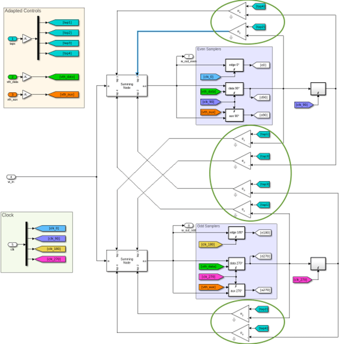
The abstract, system-level adaptation engine model, illustrated below, resides in Rx/DualSummingNodeDFECDR. The DFECDR subsystem consists of the following blocks.

1. DFE_analog – a dual-summing-node DFE

2. PD_analog – a phase detector

3. LF1 – a loop-filter

4. VCO1 – a voltage-controlled oscillator (VCO)

5. ADAPT – a DFE adaptation engine

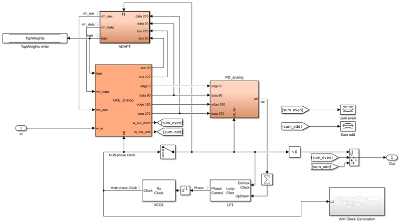
The adaptation engine in the dual-summing-node DFE model recovers the signal levels, sets the sampler thresholds, and adapts the tap weights of the DFE.

Update the Adaptation Engine for HDL Code Generation

To enable automated RTL code generation, update the abstract system-level adaptation engine model (ADAPT) with implementation-specific details. Replace the floating-point operations that are not RTL-friendly with equivalent fixed-point operations. These steps refine the abstract adaptation engine model into a bit-accurate form suitable for HDL Coder.

1. Reduce the sample rate using windowing – Change the adaptation engine processing speed from the baud rate of 50 Gbaud/s to a lower clock rate for HDL implementation.

2. Change output controls format from floating-point to integer – Change the format of the adaptation engine outputs, DFE tap weights, and sampler thresholds from floating-point to integer. Use simplified digital-to-analog converters (DACs) to convert these integer outputs to required signal levels inside the DFE.

3. Change input symbol alphabet from floating-point to integer – To enable integer-based adaption processing, update the symbol alphabet encoding in the DFE and the deserializer.

4. Update the adaptation algorithm to use integer processing – Change the adaptation algorithm to leverage bit-vectors as inputs and integer outputs and to perform processing using fixed-point (integer) arithmetic and bit-wise operations.

The following sections describe these changes in detail. The outcome of these changes is saved in the project model DualSummingNodeSerdes_bitAccurate.slx.

open_system('DualSummingNodeSerdes_bitAccurate');

Reduce Sample Rate Using Windowing

The baud rate of the system, approximately 50 Gbaud/s or 25 GHz in this half-rate system, is too high for an at-speed implementation of the adaptation engine. To decrease the speed of the adaptation logic, the adaptation engine processes a window (a group) of samples in parallel every clock cycle, instead of processing one sample in each clock cycle. The data deserialization at the DFE output accomplishes this reduction of the adaptation engine operating speed.

First, modify the adaptation loop from sample-by-sample processing to a group-of-samples processing, as shown below. Two blocks are now in the feedback path between the DFE outputs and the DFE adaptation inputs: the window-based adaptation system (ADAPT) and the de-serializer (DES).

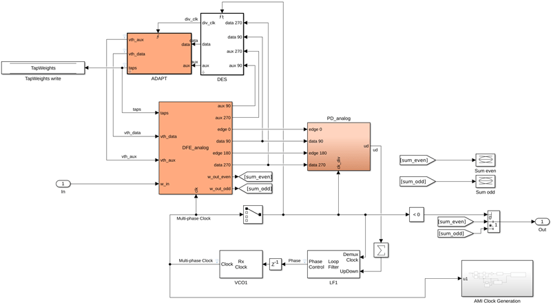
The de-serializer is typically implemented using a custom analog/digital mixed-signal design, which is why it can run at the system baud rate. To trigger the digital adaptation engine, a divided-down clock drives the digital adaptation block. The DES Simulink block, shown below, performs both functions: data de-serialization and clock division. The input and triggering logic are the same as in the sample-by-sample adaptation engine. However, rather than processing samples, the samples are shifted into a circular buffer. The DEMUX MATLAB® function block implements this circular buffer: it first stores samples in the buffer, and then it feeds a window of samples to the adaptation engine at the divided (reduced) clock rate.

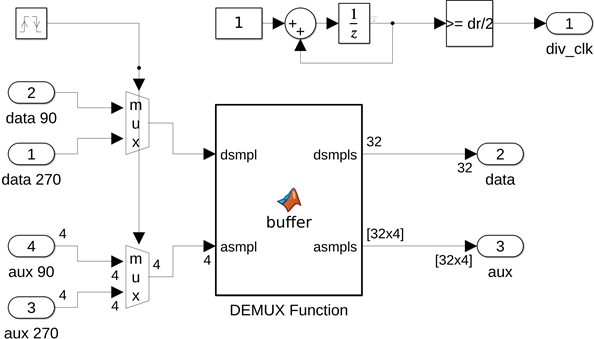
The deserialization factor is a parameter for both the de-serializer and the adaptation blocks, and it is currently set to 32, to achieve a 32:1 deserialization and clock-division ratio. The baud rate of the transceiver is 53.125 Gbaud/s, so the DFE produces a decision at a rate of 53.125 GS/s. A division ratio of 32:1 requires that the digital logic implementing the adaptation algorithm runs at 53.125 GHz/32 = 1.66 GHz. The deserialization ratio can be increased. A deserialization ratio of 64:1 yields a digital logic speed of 830 MHz at the cost of increasing the latency of the adaptation system.

With the convergence time-constants (mu parameters) used in this example, there is no appreciable difference between the convergence traces for a 32:1 or a 64:1 de-serializer setting.

Change DFE Control Format from Floating Point to Integer

Currently, the outputs from the adaptation engine are floating-point values that directly drive the DFE tap weights and sampler thresholds. However, a practical system uses a DAC to generate analog voltages from binary codewords (integer values) rather than driving the DFE with floating-point values. Next, change the output type of the adaptation engine from floating point to integer and insert DAC models into the control paths. For simplicity, use an 8b 2’s-complement codeword for both the tap-weights and the threshold-voltage controls, which can be changed to accommodate higher or lower resolutions.

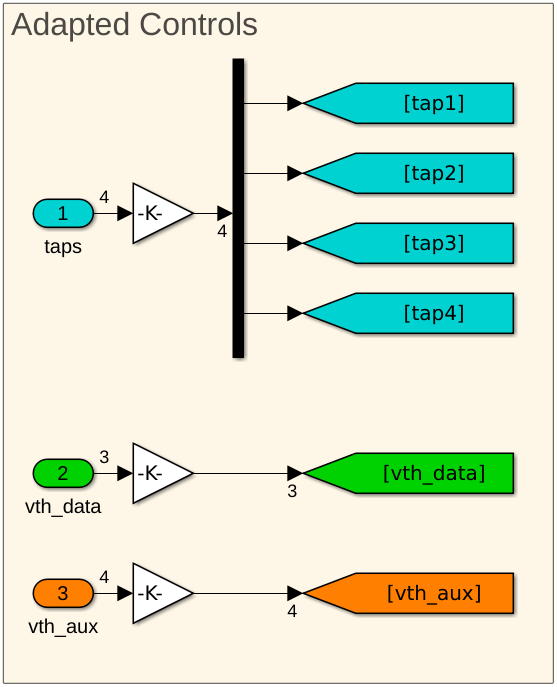
A Simulink multiplier block models the DAC: the multiplier converts the 8b 2's complement codewords into appropriately scaled voltages (floating-point controls). The tap weight gain is 0.025/128, and the threshold voltage control gain is 0.25/128. To keep the same adaptation convergence time, adjust the adaptation convergence settings, defined in the MATLAB workspace.

muTaps = muTaps * (256 * 16);
muThresholds = muThresholds * 256;

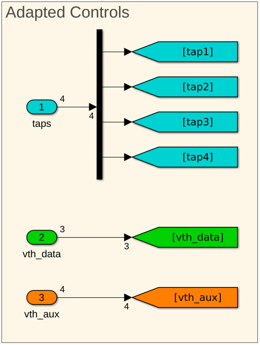
With the changes made to the muTaps and muThreshold parameters, the outputs from the adaptation block (ADAPT) are now integer scale [-128, 127], but they are not integer type. To remedy the output type of the MATLAB function:

1. Move the calculation of the vth_data threshold, into the MATLAB function.

2. Set the outputs of the function to use the int8 data type using the Property Inspector dialog box.

3. Cast the vlev and taps assignments into int8. These variables are located at the bottom of the ADAPT function.

% Data buffer
vlev = int8(vstate(1 : 4));
vdat = int8(mean([vstate(1:3), vstate(2:4)], 2));
taps = int8(tstate(1 : 4));

4. To maintain IBIS-AMI export compliance, where the DFE tap values are represented as a voltage, scale the IBIS-AMI tap weight output by the DAC gain.

Run the convergence again and observe the results. The results yield the same curves but use an integer output scale with tap and threshold voltage quantization.

Change Input-Symbol Alphabet from Floating Point to Integer

To change the algorithmic-adaptation function into an RTL-export-ready function, you need bit-accurate DFE and de-serializer outputs. Currently, the DFE outputs are 4-state floating-point values for the data samplers and 2-state floating-point 4-entry vectors for the auxiliary samplers. The 4-state symbol alphabet is from the set [-1,-1/3,+1/3,+1], which is suitable for an algorithmic adaptation function, but not a bit-accurate digital function. Similarly, the 2-state symbol alphabet is from the set [-1,+1], which is also not the required Boolean nor integer representation needed.

Change Data Sampler Output Values

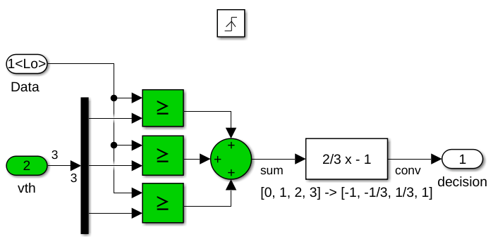
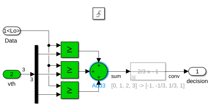
Modify the data sampler subsystems, DFE_analog/delay 8 and DFE_analog/delay 4. Change the output of the data slicers 4-state symbol alphabet from [-1,-1/3,+1/3,+1] to [0,1,2,3] by commenting through the remapping function as shown by the two figures below. Next, change the output type of the 3-input summation from a double output data type to fixdt(0,2,0), which is a 2b unsigned integer value. The data sampler is a triggered system, so use the decision block dialog box to update the initial value of the output from -1, a valid value from the [-1,-1/3,+1/3,+1] alphabet, to 0, which is a valid value in the updated output alphabet.

Change Auxiliary Sampler Output Values

Change the auxiliary sampler subsystems, DFE_analog/delay 3 and DFE_analog/delay 5, to output [0,1] (Boolean) decisions rather than [-1,1]:

1. Remove the cast to double and polynomial function blocks.

2. Combine the Boolean outputs from the 4 individual comparators into a 4b vector using a 4-input bit-concatenation block.

3. Flip the order of vth input vector so that it matches the concatenation order.

4. Change the initial decision output value from -1 to 0.

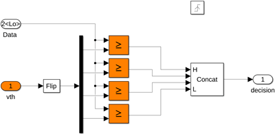
Bit concatenation is used, rather than vectorization, because the input ports for the Verilog module need to be represented as bit vectors: bit concatenation results in multi-bit RTL ports, whereas Simulink vectorization results in multiple RTL ports. Note, MATLAB equates Verilog bit vectors to fixed-point representation. A 4b vector maps to a fixdt(0,4,0) value; any 4b-wide fixed-point value would suffice. It doesn't need to be unsigned or have zero fractional bits.

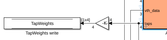
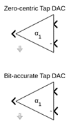
Change DFE Tap Steering Block

The DFE leverages the zero symmetry of the original symbol alphabet: [-1,-1/3,+1/3,+1]. In the DFE, sampler decisions are used in feedback, along with the DFE tap weights, to control the DFE contribution. However, the new RTL friendly decision alphabet, [0,1,2,3] is no longer zero symmetric. Change the DFE tap-steering blocks, highlighted in the figure below, to be compatible with the new decision alphabet.

The correct DFE tap-weight component, Bit-Accurate Tap DAC, is in the DFE_parts.slx library, shown below.

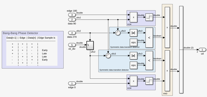
Change Data Mapping of Phase Detector

The phase detector makes use of the data decisions to drive the bang-bang phase detector. The phase detector uses the [-1,-1/3,+1/3,+1] alphabet. A picture of the original phase detector is shown below.

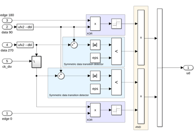
Update the phase detector using the ufix2 -> dbl component from the DFE_parts.slx library, as shown below.

Change De-serializer from Vectorization to Bit-Concatenation

The algorithmic de-serializer does the following:

• Packs 4-state data-sampler outputs into a 32-entry vector.

• Packs 4-entry 2-state data-sampler outputs into a 32 x 4 matrix.

This arrangement works well for the algorithmic model because MATLAB vector indexing can be used to process the 32 samples using a for-loop. However, the 32-entry vectors are mapped into individual input pins in the RTL module. Since the RTL signals are grouped into multi-bit busses, individual input pins are not suitable.

To achieve bussed-signal interfaces for the generated Verilog module, change the de-serializer as follows:

1. Pack the 2b data-sampler outputs, using an fixdt(0,2,0) representation, into a 32 x 2b = 64b output, fixdt(0,64,0).

2. Pack the 4b of combined auxiliary outputs, using an fixdt(0,4,0) representation, into a 32 x 4b output, fixdt(0,128,0).

The original de-serializer MATLAB function is shown below.

function [dsmpls, asmpls] = buffer(dsmpl, asmpl, dr)

persistent data aux count dsmpls_out asmpls_out
if isempty(data)
    data = zeros(dr, 1);
    dsmpls_out = zeros(dr, 1);
    
    aux = zeros(dr, length(asmpl));
    asmpls_out = zeros(dr, length(asmpl));
    
    count = uint8(0);
end


if (count == 0)
    dsmpls_out = data;
    asmpls_out = aux;
end

count = mod(count + 1, dr);

data = circshift(data, 1);
data(1) = dsmpl;
aux = circshift(aux, 1);
aux(1, 1 : length(asmpl)) = asmpl;

dsmpls = dsmpls_out(1 : dr);
asmpls = asmpls_out(1 : dr, 1 : length(asmpl));

Change the function so that it matches the function code below.

function [dsmpls, asmpls] = buffer(dsmpl, asmpl, dr)

persistent data aux count dsmpls_out asmpls_out
if isempty(data)
    aux = fi(0, 0, dr * asmpl.WordLength, 0);
    asmpls_out = fi(0, 0, dr * asmpl.WordLength, 0);
    data = fi(0, 0, dr * dsmpl.WordLength, 0);
    dsmpls_out = fi(0, 0, dr * dsmpl.WordLength, 0);
    
    count = uint8(0);
end


if (count == 0)
    dsmpls_out = data;
    asmpls_out = aux;
end

count = mod(count + 1, dr);
if (dr == 1)
    data = dsmpl;
    aux = asmpl;
else
    data = bitconcat(bitsliceget(data, (dr - 1) * dsmpl.WordLength), dsmpl);
    aux = bitconcat(bitsliceget(aux, (dr - 1) * asmpl.WordLength), asmpl);
end

dsmpls = dsmpls_out;
asmpls = asmpls_out;

Change the input and output parameters for the function:

1. Change dsample to use a fixdt(0,4,0) type.

2. Change dsamples from a size of dr, to a size of 1 using a fixdt(0,2*dr,0) type.

3. Change asample from a size of 4, to a size of 1 using a fixdt(0,4,0) type.

4. Change asamples from a size of [dr,4], to a size of 1 using a fixdt(0,4*dr,0) type.

Update Adaptation Algorithm to Use Integer Processing

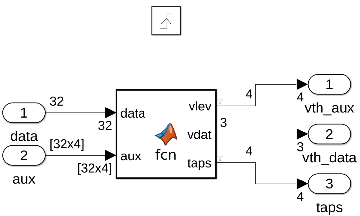
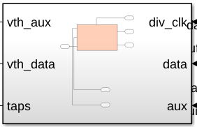
Now that the inputs and outputs from the adaptation engine are set, it is time to focus on its internal functionality. The bit-accurate functionality is shown below.

function [vlev, dlev, taps] = fcn(data, aux, int_fw, dr)


persistent vstate tstate dstate
if isempty(vstate)
    fxpt = numerictype(1, 8+int_fw, int_fw);
    vstate = fi(zeros(4, 1), fxpt, hdlfimath);
    tstate = fi(zeros(4, 1), fxpt, hdlfimath);
    dstate = fi(0, 0, 4, 0);
end

for idx = dr - 1 : -1 : 0
    d = bitsliceget(bitsrl(data, 2 * idx), 2);
    a = bitsrl(aux, 4 * idx);

    % Level restore
    if xor(bitget(a, uint8(d) + 1), bitget(d, 2))
        vstate(1 + bitxorreduce(d)) = vstate(1 + bitxorreduce(d)) + fi(fxpt.eps, fxpt, hdlfimath);
    else
        vstate(1 + bitxorreduce(d)) = vstate(1 + bitxorreduce(d)) - fi(fxpt.eps, fxpt, hdlfimath);
    end

    % Taps
    for tapidx = 1 : 4
        if xor(bitget(dstate, tapidx), bitget(a, uint8(d) + 1))
            tstate(tapidx) = tstate(tapidx) - fi(fxpt.eps, fxpt, hdlfimath);
        else
            tstate(tapidx) = tstate(tapidx) + fi(fxpt.eps, fxpt, hdlfimath);
        end
    end

    % Data buffer
    dstate = bitconcat(bitsliceget(dstate, 3), bitget(d, 2)); %% MSB
end

vlev = int8([vstate(1 : 2); -vstate(2 : -1 : 1)]);

dlev = int8(zeros(3,1));
dlev(1) = int8(bitsra(vlev(1) + vlev(2), 1));    
dlev(3) = int8(bitsra(vlev(3) + vlev(4), 1));

taps = int8(tstate(1 : 4));

Change the initial state of the triggered block outputs by double-clicking on the vth_aux, vth_data, and taps output ports. Then change the Initial output values as indicated by the table below.

Port	Initial Output
vth_aux	int8([0,0,0,0]')
vth_data	int8([0,0,0]')
taps	int8([0,0,0,0]')

Generate HDL Algorithm

Now that you converted the adaptation algorithm into a bit-accurate version, it is a candidate for RTL export. HDL Coder facilitates the export of the function.

The following sections describe the process of targeting the ADAPT subsystem, the culmination of which has been saved in the project model, DualSummingNodeSerdes_bitAccurate_for_export.slx.

open_system('DualSummingNodeSerdes_bitAccurate_for_export');

Complete Model Updates

Make these updates for HDL generation compatibility:

• HDL Coder requires that triggered blocks are in a subsystem. Select the ADAPT block and wrap it by right-clicking and choosing Subsystem & Model Reference/Create Subsystem from selection. Rename the new subsystem adapt.

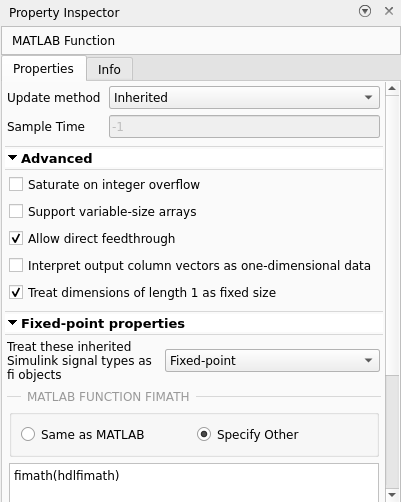
• Change the numerics for fixed point handling. Double-click the MATLAB function , adapt/ADAPT/MATLAB Function, and then select Property Inspector from the Simulation tab on the toolstrip. Clear the Saturate on integer overflow box and change Fixed-point properties from Same as MATLAB to Specify Other and then enter fimath(hdlfimath) into the text field.

Open Toolstrip and Configure Model Settings

Open the HDL Coder app from the APPS menu and follow these steps:

1. To lock in the subsystem of interest for code generation, select the adapt subsystem on the canvas, DualSummingNodeDFECDR/adapt, and pin it in the Code for box.

2. Before generating RTL code, run the HDL Code Advisor. Accept proposed fixes by clicking the hyperlinks.

3. Click Settings and make these changes:

• Change HDL Code Generation/Target/Target Frequency to 1660.

• Deselect HDL Code Generation/Global Settings/Additional Settings/Model Generation/Generated model.

• Reenable the IBIS-AMI toolchain by setting Code Generation/Build process/Toolchain to IBIS-AMI GNU gcc/g++.

• Reenable support for dynamic memory allocation by enabling Simulation Target/Advanced parameters/Dynamic memory allocation for MATLAB functions.

Generate Adapt Block HDL

The adaptation model should now be ready for export. To export the model into RTL, click Generate HDL Code from the HDL Toolbar (number 4 above).

Alternatively, you can invoke makehdl at the command line:

makehdl('DualSummingNodeSerdes_bitAccurate_for_export/Rx/DualSummingNodeDFECDR/adapt');

### Begin compilation of the model 'DualSummingNodeSerdes_bitAccurate_for_export'...
### Working on the model DualSummingNodeSerdes_bitAccurate_for_export
### Generating HDL for DualSummingNodeSerdes_bitAccurate_for_export/Rx/DualSummingNodeDFECDR/adapt
### Using the config set for model DualSummingNodeSerdes_bitAccurate_for_export for HDL code generation parameters.
### Running HDL checks on the model 'DualSummingNodeSerdes_bitAccurate_for_export'.
### Working on the model 'DualSummingNodeSerdes_bitAccurate_for_export'...
### Begin Verilog Code Generation for 'DualSummingNodeSerdes_bitAccurate_for_export'.
### Working on DualSummingNodeSerdes_bitAccurate_for_export/Rx/DualSummingNodeDFECDR/adapt/ADAPT as hdl_prj/hdlsrc/DualSummingNodeSerdes_bitAccurate_for_export/ADAPT_block.v.
### Working on DualSummingNodeSerdes_bitAccurate_for_export/Rx/DualSummingNodeDFECDR/adapt as hdl_prj/hdlsrc/DualSummingNodeSerdes_bitAccurate_for_export/adapt.v.
### Code Generation for 'DualSummingNodeSerdes_bitAccurate_for_export' completed.
### Generating HTML files for code generation report at DualSummingNodeSerdes_bitAccurate_for_export_codegen_rpt.html
### Creating HDL Code Generation Check Report adapt_report.html
### HDL check for 'DualSummingNodeSerdes_bitAccurate_for_export' complete with 0 errors, 1 warnings, and 0 messages.
### HDL code generation complete.

Once the process is complete, open the generated top-level design RTL:

open hdl_prj/hdlsrc/DualSummingNodeSerdes_bitAccurate_for_export/adapt.v

Notice the following:

1. The RTL interface consists of a minimum set of interface ports.

module adapt
          (reset,
           div_clk,
           data,
           aux,
           vth_aux_0,
           vth_aux_1,
           vth_aux_2,
           vth_aux_3,
           vth_data_0,
           vth_data_1,
           vth_data_2,
           taps_0,
           taps_1,
           taps_2,
           taps_3);

2. The decisions from the DFE, data and aux, are provided as a bit vector.

input   [63:0] data;  // ufix64
input   [127:0] aux;  // ufix128

Verify Generated HDL Algorithm

This example includes a testbench to simulate the Verilog model.

Choose HDL Simulator

Use HDL Coder to generate RTL for the adaptation engine. Then, run the adaptation-engine HDL using your choice of HDL simulator, with inputs saved from a Simulink run of the adaptation engine.

% This is a MathWorks-specific setup. You must assign PATH and
% other settings specific to your environment for your chosen simulator.
setup_questa();

% Uncomment one of the following supported HDL simulator choices:
current_hdl_simulator = 'Questa'; % Windows or Linux
% current_hdl_simulator = 'Xcelium'; % Linux only
% current_hdl_simulator = 'VCS'; % Linux only
% current_hdl_simulator = 'Vivado'; % Linux only

Run Simulink and Verilog to Compare Results

Run the Simulink vs. Verilog comparison script, which performs the following actions:

1. Runs the Simulink simulation and captures the adaptation block inputs and outputs.

2. Writes the adaptation block inputs into binary files for use by the Verilog simulation.

3. Runs the Verilog simulation, using the generated RTL code and the stimulus saved by Simulink.

4. Reads in the Verilog outputs.

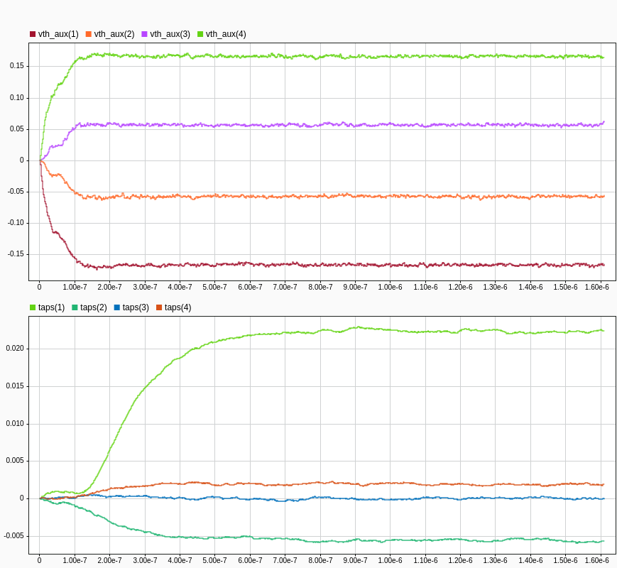
5. Plots the Simulink and Verilog adaptation outputs.

compare_simulation

Reading pref.tcl

# 2023.2

# do scripts/tb_tran_questa.do
# QuestaSim-64 vlog 2023.2 Compiler 2023.04 Apr 11 2023
# Start time: 18:42:11 on Jan 13,2024
# vlog -sv hdl_prj/hdlsrc/DualSummingNodeSerdes_bitAccurate_for_export/adapt.v 
# -- Compiling module adapt
# 
# Top level modules:
# 	adapt
# End time: 18:42:11 on Jan 13,2024, Elapsed time: 0:00:00
# Errors: 0, Warnings: 0
# QuestaSim-64 vlog 2023.2 Compiler 2023.04 Apr 11 2023
# Start time: 18:42:11 on Jan 13,2024
# vlog -sv hdl_prj/hdlsrc/DualSummingNodeSerdes_bitAccurate_for_export/ADAPT_block.v 
# -- Compiling module ADAPT_block
# 
# Top level modules:
# 	ADAPT_block
# End time: 18:42:11 on Jan 13,2024, Elapsed time: 0:00:00
# Errors: 0, Warnings: 0
# QuestaSim-64 vlog 2023.2 Compiler 2023.04 Apr 11 2023
# Start time: 18:42:12 on Jan 13,2024
# vlog -sv hdl_tb/adapt_tb.v 
# -- Compiling module adapt_tb
# 
# Top level modules:
# 	adapt_tb
# End time: 18:42:12 on Jan 13,2024, Elapsed time: 0:00:00
# Errors: 0, Warnings: 0
# vsim -c work.adapt_tb 
# Start time: 18:42:12 on Jan 13,2024
# ** Note: (vsim-3812) Design is being optimized...
# //  Questa Sim-64
# //  Version 2023.2 linux_x86_64 Apr 11 2023
# //
# //  Copyright 1991-2023 Mentor Graphics Corporation
# //  All Rights Reserved.
# //
# //  QuestaSim and its associated documentation contain trade
# //  secrets and commercial or financial information that are the property of
# //  Mentor Graphics Corporation and are privileged, confidential,
# //  and exempt from disclosure under the Freedom of Information Act,
# //  5 U.S.C. Section 552. Furthermore, this information
# //  is prohibited from disclosure under the Trade Secrets Act,
# //  18 U.S.C. Section 1905.
# //
# Loading sv_std.std
# Loading work.adapt_tb(fast)
# ** Note: $finish    : hdl_tb/adapt_tb.v(55)
#    Time: 2051 ns  Iteration: 1  Instance: /adapt_tb
# End time: 18:42:13 on Jan 13,2024, Elapsed time: 0:00:01
# Errors: 0, Warnings: 0

The plots show that the Simulink-based adaptation and RTL code for it behave the same between the two environments.

Conclusion

The generated RTL can be directly used in Verilog simulations to build or validate larger systems. The generated code can also be used as input into a synthesis engine. Furthermore, refinements to the exported code can be made in MATLAB or Simulink to improve upon its resource utilization and parallelization of operations. This example highlights a path towards generating synthesizable code directly from a SerDes Toolbox model. The example refines an abstract system-level model into a bit-accurate representation of the adaptation engine while maintaining IBIS-AMI export capabilities.

Reference

[1] S. Ibrahim and B. Razavi, "Low-Power CMOS Equalizer Design for 20-Gb/s Systems," in IEEE Journal of Solid-State Circuits, vol. 46, no. 6, pp. 1321-1336, June 2011, doi: 10.1109/JSSC.2011.2134450.