Wind Turbine Driveline with Vibrations

This example shows a wind turbine rotor, controller, and flexible drive shaft with transverse vibrations. Click the button below to open the model.

 
open_system('WindTurbineDrivelineWithVibrations')

Example Overview

This example contains a wind turbine rotor, controller, and flexible shaft with transverse vibrations. The direct-drive wind turbine has a power capacity of 10 MW. Controllers based on the NREL 5-MW reference wind turbine adjust the generator torque and collective blade pitch. The rotor and shaft are supported by 4 fluid film bearings. This example lets you optionally model transverse vibrations of the driveshaft due to a generator unbalanced magnetic force. The rotor dynamics can be modeled using a lumped mass finite element method or a reduced order model to simulate the shaft vibrations more efficiently. The reduced order models include a traditional static eigenmodes method and a speed-dependent eigenmodes method. This example includes scripts for analyzing the performance of the different reduced order models.

 
open_system('WindTurbineDrivelineWithVibrations')

Aerodynamics

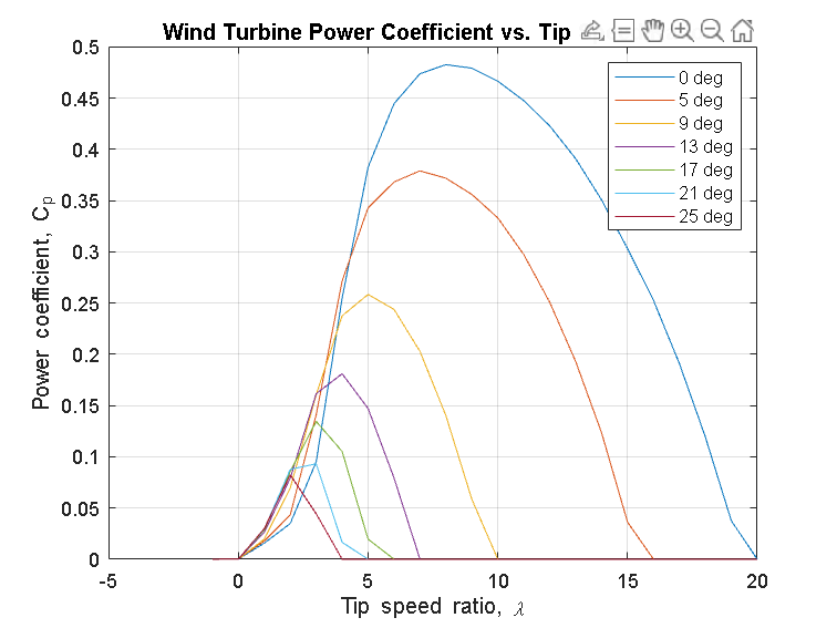
Rotor torque as a function of wind speed and blade pitch is modeled using a Wind Turbine block from Simscape™ Driveline™. The block models torque quasi-statically based on the wind turbine power coefficient curves and rotor speed.

 

% Retrieve the model data
hws= get_param('WindTurbineDrivelineWithVibrations', 'modelworkspace');
rotor= getVariable(hws, 'rotor');

% Generate the plot
figure;
hold on
for i=1:length(rotor.pitch)
    plot(rotor.TSR, rotor.Cp(i,:), 'DisplayName', [num2str(rotor.pitch(i)) ' deg'])
end
box on
grid on
legend show
title('Wind Turbine Power Coefficient vs. Tip Speed Ratio')
xlabel('Tip speed ratio, \lambda')
ylabel('Power coefficient, C_p');

Controllers & Braking

Controllers for the 10 MW wind turbine are configured for the direct-drive rotation speeds and scaled up from the NREL 5-MW reference wind turbine described in Jonkman, J.; Butterfield, S.; Musial, W.; Scott, G., Definition of a 5-MW reference wind turbine for offshore system development (No. NREL/TP-500-38060). National Renewable Energy Lab. Golden, CO, USA, 2009.

The generator torque controller starts producing torque when the rotor speed exceeds the cut-in speed. When the generator power is less than the rated power, torque is a function of the generator speed. The torque values are chosen to maximize power. This example models this torque using a Lookup Table. When the power equals the rated power, the generator torque adjusts based on rotor speed to maintain the rated power. This example switches between the below-rated and above-rated torque generation modes using a Switch block. The Switch block switching criteria represents the rated power threshold via a blade pitch sensor: the collective blade pitch controller causes the blade pitch to exceed 1 deg when the rated power has been reached.

This model implements the generator torque using an Ideal Torque Source block. The model accounts for drivetrain losses as a simple rotational damper. Rotational Power Sensor and Ideal Rotational Motion Sensor blocks sense the generator power and speed, respectively. Generated mechanical power exceeds 10 MW before electrical losses are taken into account.

 
open_system('WindTurbineDrivelineWithVibrations/Controlled Generator')

The collective blade pitch controller begins adjusting the blade pitch once the rated turbine speed is reached. The controller is a PI controller that tries to maintain the rated turbine speed. The proportional and integral coefficients are scheduled functions of the blade pitch. The blade pitch responds instantaneously to the controller command without accounting for inertial dynamics.

 
open_system('WindTurbineDrivelineWithVibrations/Pitch Controller')

When the wind speed exceeds the turbine's maximum wind speed, a brake is activated.

 
open_system('WindTurbineDrivelineWithVibrations/Brake')

Simulation Results from Scopes

The scope shows the generated power, rotational velocity, and blade pitch response to the wind speed. Once the turbine rotational velocity exceeds a start-up threshold, the power generation begins. Once the rated power is reached, the blade pitch begins increasing to maintain the rated power.

  
open_system('WindTurbineDrivelineWithVibrations');
set_param('WindTurbineDrivelineWithVibrations/Scope','open','on');
out= sim('WindTurbineDrivelineWithVibrations'); %#ok<NASGU>

clear out

Simulation Results from Simscape Logging

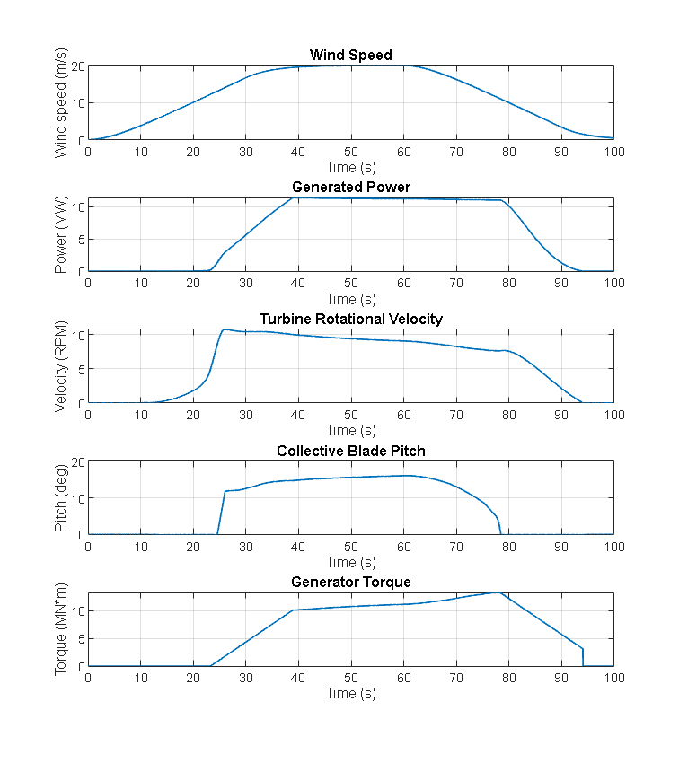
The script below uses results from Simscape logging to plot the wind speed, generated power, turbine rotational velocity, blade pitch, and generator torque in a figure. When the wind speed increases above the rated wind speed, the blade pitch increases to limit the aerodynamic power. When the turbine rotational velocity decreases in response to the increased blade pitch, the generator torque increases to maintain the rated power. When the wind speed decreases, the pitch controller decreases the blade pitch, and the turbine rotational velocity decreases at a faster rate. The generator torque decreases when the generated power is below the rated power.

 
WindTurbineDrivelineWithVibrationsPlotControlledPower;

% Uncomment the line below to see the code for generating the figure.
% edit WindTurbineDrivelineWithVibrationsPlotControlledPower;

Rotor Dynamics

This example lets you optionally model transverse vibrations of the driveshaft due to a generator unbalanced magnetic force. The Flexible Shaft block models varied shaft diameters, rigid inertias, and fluid film bearings along shaft. The example models the blades, hub, and generator rotor as rigid inertias.

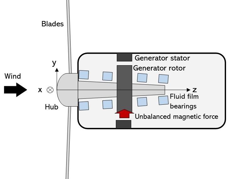
Wind turbine driveline schematic

The Shaft subsystem separates the rigid rotational dynamics that drive the wind turbine and the flexible shaft vibration dynamics. The Ideal Rotational Motion Sensor, PS Gain, and Ideal Angular Velocity Source blocks excite the transverse dynamics at a harmonic of the shaft speed.

 
set_param('WindTurbineDrivelineWithVibrations/Shaft', 'vibration_model', 'Lumped mass');
open_system('WindTurbineDrivelineWithVibrations/Shaft/Lumped mass');
open_system('WindTurbineDrivelineWithVibrations/Shaft/Lumped mass/Shaft');

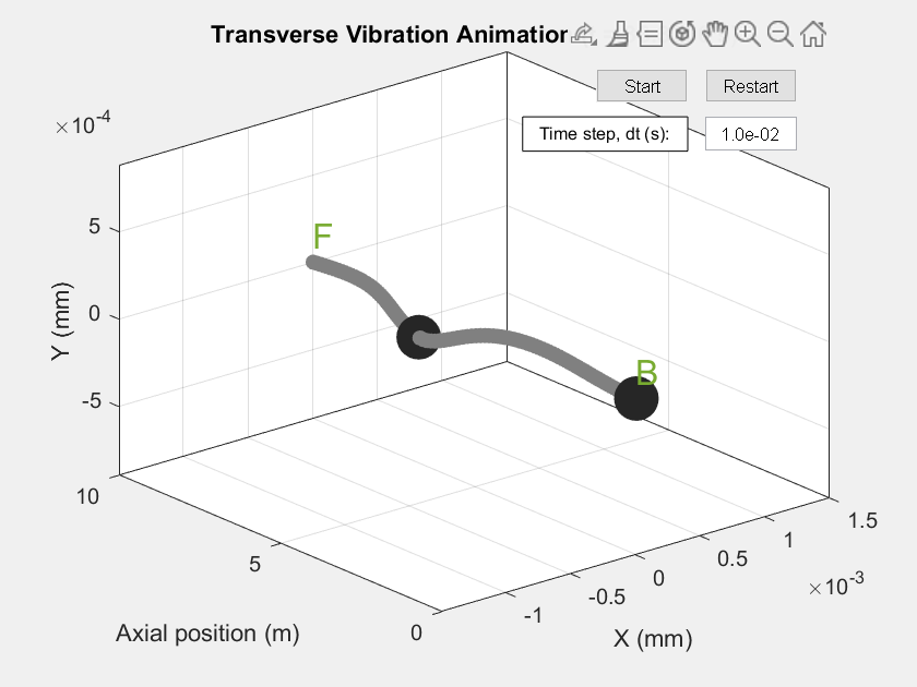
Click the button below to simulate the model and run an animation of the shaft transverse vibrations. The button generates a standalone figure for running the animation. The image below is a screenshot of the animation.

 
set_param('WindTurbineDrivelineWithVibrations/Shaft', 'vibration_model', 'Speed-dependent eigenmodes');
WindTurbineDrivelineWithVibrationsAnimate;

% Uncomment the line below to see the code for generating the figure.
% edit WindTurbineDrivelineWithVibrationsAnimate;

Rotor Dynamics Analysis Workflow

The Flexible Shaft block can model the driveshaft transverse vibrations using a speed-dependent eigenmodes method that adjusts the modal properties as the shaft speed changes.

The script below plots the shaft eigen mode shapes and frequencies for varied shaft speeds. Modes with large displacements at the axial locations excited by external loadings and modes with natural frequencies equal to the shaft speed or external loading frequencies will have larger vibration responses, and you generally want to avoid designs with these characteristics. The button generates a standalone figure for plotting the mode shapes. The image below is a screenshot of the figure.

 
set_param('WindTurbineDrivelineWithVibrations/Shaft', 'vibration_model', 'Speed-dependent eigenmodes');
clear flex_shaft_mode_props % clear any existing mode properties
WindTurbineDrivelineWithVibrationsPlotEigenmodes;

% Uncomment the line below to see the code for generating the app.
% edit WindTurbineDrivelineWithVibrationsPlotEigenmodes

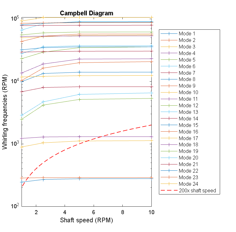
Click the button below to view the Campbell frequency analysis plot for the flexible shaft.

 
set_param('WindTurbineDrivelineWithVibrations/Shaft', 'vibration_model', 'Speed-dependent eigenmodes');
WindTurbineDrivelineWithVibrationsPlotCampbellDiagram;

% Uncomment the line below to see the code for generating the figure.
% edit WindTurbineDrivelineWithVibrationsPlotCampbellDiagram

Reduced Order Model Workflow

Rotor dynamics for the flexible shaft with speed-dependent bearings and rigid inertias can be modeled using a lumped mass finite element method or a more computationally efficient reduced order model. The reduced order models for simulating the transverse vibrations include a traditional static eigenmodes method and a speed-dependent eigenmodes method.

The lumped mass model for the flexible shaft transverse vibrations divides the shaft into linear finite elements with inertias centered at nodes. Each node has four degrees of freedom: two translational motions and two rotational motions. The two reduced order models are reductions of the lumped mass model.

The static eigenmode method computes the eigenmodes of the shaft-bearing-disk system at a nominal shaft speed. The method simulates the modal degrees of freedom rather than the node degrees of freedom. Since the number of modal degrees of freedom << the number of node degrees of freedom, the eigenmode model reduction significantly speeds up the simulation. The static eigenmode method does not adjust modal properties as the shaft speed changes, so large gyroscopic effects and changes in bearing properties with shaft speed limit simulation accuracy.

The speed-dependent eigenmode method computes the eigenmodes of the shaft-bearing-disk system at varied reference shaft speeds. During the simulation, the model updates the modal properties as speed-dependent gyroscopic and bearing properties change to improve simulation accuracy.

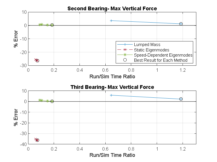
Click the button below to compare the performance of the different reduced order models with varied settings.

 
% This script simulates the model multiple times using the three different
% vibration modeling methods and plots the computational performance.
WindTurbineDrivelineWithVibrationsPerformanceComparison;

Getting rigid results
Simulation 1 of 1
Execution time: 1: 0.21315 s
Getting Lumped mass results
Simulation 1 of 2. 5 flexible elements
Execution time: 61.1447 s
Simulation 2 of 2. 10 flexible elements
Execution time: 87.1059 s
Getting Static eigenmodes results
Simulation 1 of 4. 12 modes
Execution time: 9.0953 s
Simulation 2 of 4. 16 modes
Execution time: 10.4923 s
Simulation 3 of 4. 20 modes
Execution time: 10.2573 s
Simulation 4 of 4. 24 modes
Execution time: 13.2137 s
Getting Speed-dependent eigenmodes results
Simulation 1 of 4. 12 modes
Execution time: 12.2347 s
Simulation 2 of 4. 16 modes
Execution time: 13.0198 s
Simulation 3 of 4. 20 modes
Execution time: 18.2771 s
Simulation 4 of 4. 24 modes
Execution time: 20.1047 s

% Uncomment the line below to see the code for generating the figure.
% edit WindTurbineDrivelineWithVibrationsPerformanceComparison

You can adjust lines 36-41 in WindTurbineDrivelineWithVibrationsPerformanceComparison.m to investigate the effects of increased lumped elements and modes.