Satellite Visibility Analysis Using Terrain

Since R2025a

This example shows how to analyze satellite visibility from a ground station using a visibility mask computed from the surrounding terrain. A visibility mask is a set of azimuth and elevation angles that define where obstructions block a satellite's line-of-sight visibility.

By combining the mapping capabilities in Mapping Toolbox™ with the satellite scenario capabilities in Satellite Communications Toolbox, you can compute visibility masks using terrain elevation data and use the masks for satellite access or link analysis. This example shows you how to:

• Load and visualize terrain elevation data in the area of interest (AOI) surrounding a ground station.

• Compute and visualize a visibility mask for the ground station using terrain elevation data.

• Visualize animated satellite sky tracks with a visibility mask using a satellite scenario object and the skyplot function.

• Create a satellite visibility chart, including visibility with the mask and without the mask.

Define Ground Station Coordinates

Define the ground station latitude, longitude, and antenna height (in meters) above ground level.

lat0 = 40.000;   % Latitude (degrees)
lon0 = -105.250; % Longitude (degrees)
h0AGL = 1.7;     % Antenna height above ground level (meters)

Load and Visualize Terrain Elevation Data

Terrain elevation data is required to compute a visibility mask for the ground station. Load and visualize terrain elevation data in an AOI surrounding the ground station.

Define AOI for Ground Station

Define a circular AOI centered at the ground station with a radius of 100 km. To ensure that the visibility mask is accurate, specify a radius that includes all surrounding terrain that can impact visibility from the ground station.

r = 100000; % 100 km
rdeg = km2deg(r/1000);
aoi = aoicircle(lat0,lon0,rdeg);

Read Terrain Elevation Data for AOI

Read terrain elevation data for the AOI from a Web Map Service (WMS) server. WMS servers provide geospatial data such as elevation, temperature, and weather from web-based sources.

Get geographic limits of the AOI.

[latlim,lonlim] = bounds(aoi);

Define the sample spacing and the corresponding cell size for the terrain data.

terrainSampleSpacing = 100; % meters
cellSize = km2deg(terrainSampleSpacing/1000);

Search the WMS Database for terrain elevation data hosted by MathWorks®. The wmsfind function returns search results as layer objects. A layer is a data set that contains a specific type of geographic information, in this case, the elevation data.

layer = wmsfind("mathworks",SearchField="serverurl");
layer = refine(layer,"elevation");

Read the elevation data from the layer into the workspace as an array and a raster reference object in geographic coordinates. Specify the image format as BIL to get quantitative data.

[Z,R] = wmsread(layer,Latlim=latlim,Lonlim=lonlim, ...
    ImageFormat="image/bil",CellSize=cellSize);

Prepare the elevation data for plotting by converting the data type to double.

Z = double(Z);

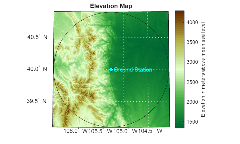
Visualize AOI and Terrain

Visualize the ground station and AOI on a 2-D map with terrain elevation data.

Visualize the terrain elevation data on a map with an appropriate colormap. Prepare to plot additional data on the map by returning the map object as h.

figure
h = usamap(Z,R);
geoshow(Z,R,DisplayType="texturemap")
demcmap(Z)

Create a geospatial table from the AOI. Then, visualize the AOI on the map.

Shape = aoi;
GT = table(Shape);
geoshow(GT,FaceAlpha=0)

Visualize the ground station on the map.

geoshow(lat0,lon0,DisplayType="point",...
    MarkerEdgeColor="k", ...
    MarkerFaceColor="c", ...
    MarkerSize=6,Marker="o")
textm(lat0,lon0+.05,"Ground Station",Color="c")

Add a title and labeled color bar.

title("Elevation Map");
cb = colorbar;
cb.Label.String = "Elevation in meters above mean sea level";

Compute and Plot Visibility Mask

Compute a visibility mask using terrain and then plot it on a 2-D polar axes, a 2-D map, and a 3-D globe. The visibility mask is a set of azimuth and elevation angles that define where the terrain blocks a satellite's line-of-sight visibility. Azimuth angles are measured clockwise from north.

Compute Visibility Mask Using Terrain

Compute the visibility mask by measuring the maximum elevation angles to terrain elevation along radial tracks from the ground station.

Specify the azimuth angles of the visibility mask.

numaz = 720;
maskaz = linspace(0,360,numaz);

For each azimuth angle, compute latitude-longitude tracks from the ground station to the boundary of the AOI.

wgs84 = wgs84Ellipsoid;
trackradius = r*ones(size(maskaz));
numtrackpts = floor(r/terrainSampleSpacing);
[tracklat,tracklon] = track1(lat0,lon0,maskaz',trackradius',wgs84,"degrees",numtrackpts);

Convert the terrain elevation data from orthometric height to ellipsoidal height referenced in the WGS84 ellipsoid. Ellipsoidal height enables better geometric accuracy than orthometric height.

[Zlat,Zlon] = geographicGrid(R);
N = egm96geoid(Zlat,Zlon);
Zwgs84 = Z + N;

Compute the ellipsoidal heights of the ground station antenna and the track points.

h0wgs = geointerp(Zwgs84,R,lat0,lon0);
h0 = h0wgs + h0AGL;
trackheight = geointerp(Zwgs84,R,tracklat,tracklon);

For each track point, compute the elevation angle and the range from the ground station.

[~,trackElevationAngles,trackrange] = geodetic2aer(tracklat,tracklon,trackheight,lat0,lon0,h0,wgs84);

Compute the maximum elevation angle from the ground station to the track points to get the elevation angles for the visibility mask.

[maskel,maskelind] = max(trackElevationAngles);

Plot Visibility Mask on a 2-D Polar Axes

Create a polar plot of the visibility mask. Apply the Mapping Toolbox convention for the azimuth direction.

figure
polarplot(deg2rad(maskaz),maskel)

ax = gca;
ax.ThetaDir = "clockwise";
ax.ThetaZeroLocation = "top";
title("Visibility Mask Using Terrain");

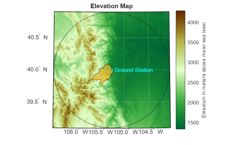
Plot Visibility Mask on a 2-D Map

Plot the visibility mask on a 2-D map using an arbitrary scale factor. You can use an arbitrary scale factor because the shape of the mask illustrates the relative degree to which the terrain blocks the visibility in each direction. As a result, the absolute size of the visibility mask is not physically meaningful.

Calculate the maximum elevation angle of the mask. Then, find the azimuth and range of the point that corresponds to the maximum elevation angle.

[maxmaskel,maxelind] = max(maskel);
maxmaskaz = maskaz(maxelind);
maskrange = trackrange(maskelind);
maxmaskrange = maskrange(maxelind);

Plot the visibility mask on a 2-D map using a geographic polygon shape. Scale the size of the visibility mask using an arbitrary scale factor of 4000.

[masklat,masklon] = aer2geodetic(maskaz,0,4000*maskel,lat0,lon0,h0,wgs84);
Shape = geopolyshape(masklat,masklon);
GT = table(Shape);
geoshow(h,GT,FaceAlpha=0.7)

Plot Visibility Mask on a 3-D Geographic Globe

Plot the visibility mask on a 3-D globe. Scale the plot so that the boundary of the mask touches the terrain point with the maximum elevation angle from the ground station.

Create a geographic globe and visualize the ground station.

gl = geoglobe(uifigure);

geoplot3(gl,lat0,lon0,h0,HeightReference="ellipsoid", ...
    LineStyle="none",Marker="o",Color="magenta", ...
    MarkerSize=1,LineWidth=4)
hold(gl,"on")

Visualize the 3-D visibility mask by plotting the boundary of the mask and by plotting lines from the ground station. Calculate the geodetic coordinates of the lines by converting the azimuth, elevation, and range values of the mask to latitude, longitude, and height. Instead of using an arbitrary scale factor, specify the scale using the range of the maximum elevation angle of the mask.

[masklat3d,masklon3d,maskh] = aer2geodetic(maskaz,maskel,maxmaskrange,lat0,lon0,h0,wgs84);
maskplotlat = [];
maskplotlon = [];
maskploth = [];
for maxelind=1:20:numel(masklat3d)
    maskplotlat = [maskplotlat lat0 masklat3d(maxelind) NaN]; %#ok<AGROW>
    maskplotlon = [maskplotlon lon0 masklon3d(maxelind) NaN]; %#ok<AGROW>
    maskploth = [maskploth h0 maskh(maxelind) NaN]; %#ok<AGROW>
end

geoplot3(gl,maskplotlat,maskplotlon,maskploth,HeightReference="ellipsoid", ...
    Color="green",LineWidth = 1)
geoplot3(gl,masklat3d,masklon3d,maskh,HeightReference="ellipsoid", ...
    Color="green",LineWidth = 1)

Set the camera position to point toward the maximum elevation angle of the mask.

[camlat,camlon,camh] = aer2geodetic(maxmaskaz+180,maxmaskel,maxmaskrange,lat0,lon0,h0,wgs84);
campos(gl,camlat,camlon,camh)
camheading(gl,maxmaskaz)
campitch(gl,0)

Compute and Plot Satellite Visibility

Compute and visualize satellite sky tracks from the ground station to a low Earth orbit (LEO) satellite constellation. Compute and plot satellite visibility from the ground station using access analysis and the visibility mask.

Compute Satellite Sky Tracks

Compute satellite sky tracks using a satellite scenario.

Create a satellite scenario containing a low Earth orbit (LEO) satellite constellation.

sc = satelliteScenario;
sats = satellite(sc,"leoSatelliteConstellation.tle");

Add a ground station to the scenario.

gs = groundStation(sc,lat0,lon0,Altitude=h0);

Simulate the scenario for 30 minutes with a sample time of 10 seconds

sc.StopTime = sc.StartTime + minutes(30);
sc.SampleTime = 10;

Compute the azimuth and elevation angles for the satellite sky tracks.

[satazs,satels,~,timeHistory] = aer(gs,sats);

Visualize Animated Sky Plot with Visibility Mask

Process the visibility mask and sky track data for use with the skyplot function. Then, create an animated plot.

Process the visibility mask by removing negative values and the last value so that the vector length is one less than the number of mask azimuth edges.

maskel = max(maskel,0);
maskel = maskel(1:end-1);

Process the sky track data by removing negative values.

satels(satels < 0) = missing; 
satazData = satazs';
satelData = satels';

Create and animate a sky plot using the sky track and visibility mask data.

f = figure;
maskh = skyplot(satazData,satelData,sats.Name, ...
    MaskAzimuthEdges=maskaz, ...
    MaskElevation=maskel);

for maxelind = 1:size(satazData,1)
    set(maskh,AzimuthData=satazData(1:maxelind,:),ElevationData=satelData(1:maxelind,:));
    drawnow
end

Compute Satellite Visibility Using Visibility Mask

Compare satellite visibility when you ignore the terrain and when you account for the terrain.

Compute the satellite visibility. To ignore the terrain, compute the access status by setting the mask elevation angle of the ground station to 0 degrees.

gs.MaskElevationAngle = 0;
acc = access(sats,gs);
vizIgnoringTerrain = accessStatus(acc);

Compute the satellite visibility again. To account for the terrain, use the elevation angles of the ground station mask.

updateMask(gs,MaskAzimuthEdges=maskaz,MaskElevationAngle=maskel);
vizWithTerrain = accessStatus(acc);

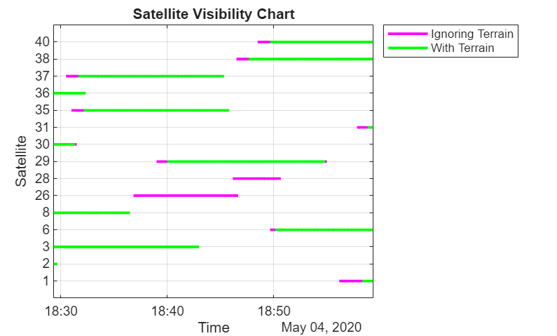
Create Satellite Visibility Chart

Create a satellite visibility chart that shows the time history of satellites.

Prepare the access status data for plotting by converting the data type to double.

vizIgnoringTerrain = double(vizIgnoringTerrain);
vizWithTerrain = double(vizWithTerrain);

Remove the satellites that are never visible.

vizIgnoringTerrain(vizIgnoringTerrain == 0) = NaN;
vizWithTerrain(vizWithTerrain == 0) = NaN;

satind = (1:size(vizIgnoringTerrain,1))';
nevervisible = all(isnan(vizIgnoringTerrain),2);

satind(nevervisible) = [];
vizIgnoringTerrain(nevervisible,:) = [];
vizWithTerrain(nevervisible,:) = [];

Plot the satellite visibility with terrain and without terrain. Observe that many satellites have times when they are obstructed by terrain. Two satellites (26 and 28) are entirely obstructed by terrain.

figure
plotind = (1:numel(satind))';
p1 = plot(timeHistory,plotind.*vizIgnoringTerrain,Color="m",LineWidth=2);
xlim([timeHistory(1) timeHistory(end)])
ylim([min(plotind)-1 max(plotind)+1])
xlabel("Time")
ylabel("Satellite")
title("Satellite Visibility Chart")
yticks(plotind)
yticklabels(satind)
grid on

hold on
p2 = plot(timeHistory,plotind.*vizWithTerrain,Color="g",LineWidth=2);
legend([p1(1) p2(1)],["Ignoring Terrain","With Terrain"],Location="northeastoutside")