Robust MIMO Controller for Two-Loop Autopilot
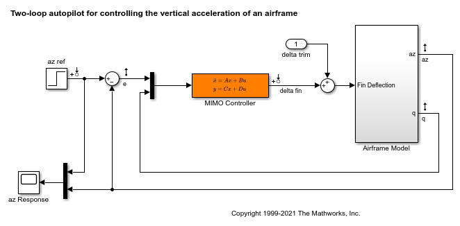
This example shows how to design a robust controller for a two-loop autopilot that controls the pitch rate and vertical acceleration of an airframe. The controller is robust against gain and phase variations in the multichannel feedback loop.
Linearized Airframe Model
The airframe dynamics and the autopilot are modeled in Simulink®. See Tuning of a Two-Loop Autopilot for more information about this model and for additional design and tuning options.
open_system('rct_airframe2')
As in the example Tuning of a Two-Loop Autopilot, trim the airframe for  and
and  . The trim condition corresponds to zero normal acceleration and pitching moment (
 and
and  steady). Use
 findop to compute the corresponding operating condition. Then, linearize the airframe model at this trim condition.
opspec = operspec('rct_airframe2');

% Specify trim condition
% Xe,Ze: known, not steady
opspec.States(1).Known = [1;1];
opspec.States(1).SteadyState = [0;0];
% u,w: known, w steady
opspec.States(3).Known = [1 1];
opspec.States(3).SteadyState = [0 1];
% theta: known, not steady
opspec.States(2).Known = 1;
opspec.States(2).SteadyState = 0;
% q: unknown, steady
opspec.States(4).Known = 0;
opspec.States(4).SteadyState = 1;
% controller states unknown, not steady
opspec.States(5).SteadyState = [0;0];

op = findop('rct_airframe2',opspec);
G = linearize('rct_airframe2','rct_airframe2/Airframe Model',op);
G.InputName = 'delta';
G.OutputName = {'az','q'};
 Operating point search report:
---------------------------------

opreport =


 Operating point search report for the Model rct_airframe2.
 (Time-Varying Components Evaluated at time t=0)

Operating point search completed successfully using optimization.
States:
----------
    Min          x          Max        dxMin        dx         dxMax
___________ ___________ ___________ ___________ ___________ ___________

(1.) rct_airframe2/Airframe Model/Aerodynamics & Equations of Motion/ Equations of Motion (Body Axes)/Position
     0           0           0         -Inf         984         Inf
-3047.9999  -3047.9999  -3047.9999     -Inf          0          Inf
(2.) rct_airframe2/Airframe Model/Aerodynamics & Equations of Motion/ Equations of Motion (Body Axes)/Theta
     0           0           0         -Inf     -0.0097235      Inf
(3.) rct_airframe2/Airframe Model/Aerodynamics & Equations of Motion/ Equations of Motion (Body Axes)/U,w
    984         984         984        -Inf       22.6897       Inf
     0           0           0           0      2.4587e-11       0
(4.) rct_airframe2/Airframe Model/Aerodynamics & Equations of Motion/ Equations of Motion (Body Axes)/q
   -Inf     -0.0097235      Inf          0      -1.7215e-16      0
(5.) rct_airframe2/MIMO Controller
   -Inf     0.00065361      Inf        -Inf     -0.0089973      Inf
   -Inf     3.7592e-20      Inf        -Inf      0.030259       Inf

Inputs:
----------
   Min         u         Max
__________ __________ __________

(1.) rct_airframe2/delta trim
   -Inf    0.00043574    Inf

Outputs: None
----------
Nominal Controller Design
Design an H-infinity controller that responds to a step change in vertical acceleration under 1 second. Use a mixed-sensitivity formulation with a lowpass weight wS that penalizes low-frequency tracking error and a highpass weight wT that enforces adequate roll-off. Build an augmented plant with azref,delta as inputs and the filtered wS*e,wT*az,e,q as outputs. (For information about the mixed-sensitivity formulation, see Mixed-Sensitivity Loop Shaping.)
sb = sumblk('e = azref-az');
wS = makeweight(1e2,5,0.1);
wS.u = 'e';
wS.y = 'we';
wT = makeweight(0.1,50,1e2);
wT.u = 'az';
wT.y = 'waz';

Paug = connect(G,wS,wT,sb,{'azref','delta'},{'we','waz','e','q'});
Compute the optimal H-infinity controller using hinfsyn. In this configuration there are two measurements e,q and one control delta.
[Knom,~,gam] = hinfsyn(Paug,2,1);
gam
gam =

    0.5928
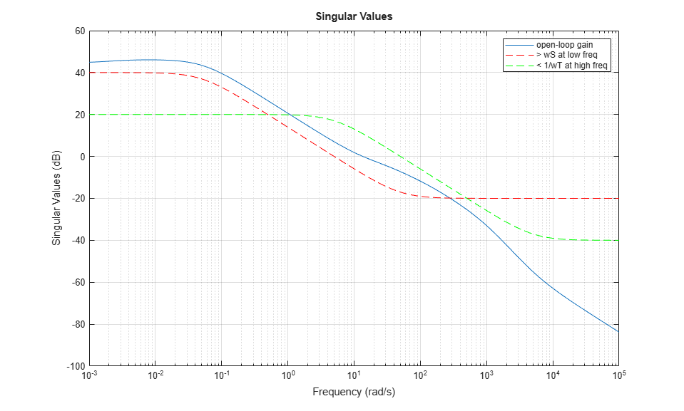
Verify the open-loop gain against wS,wT.
f = figure();
sigma(Knom*G,wS,'r--',1/wT,'g--'), grid
legend('open-loop gain','> wS at low freq','< 1/wT at high freq')
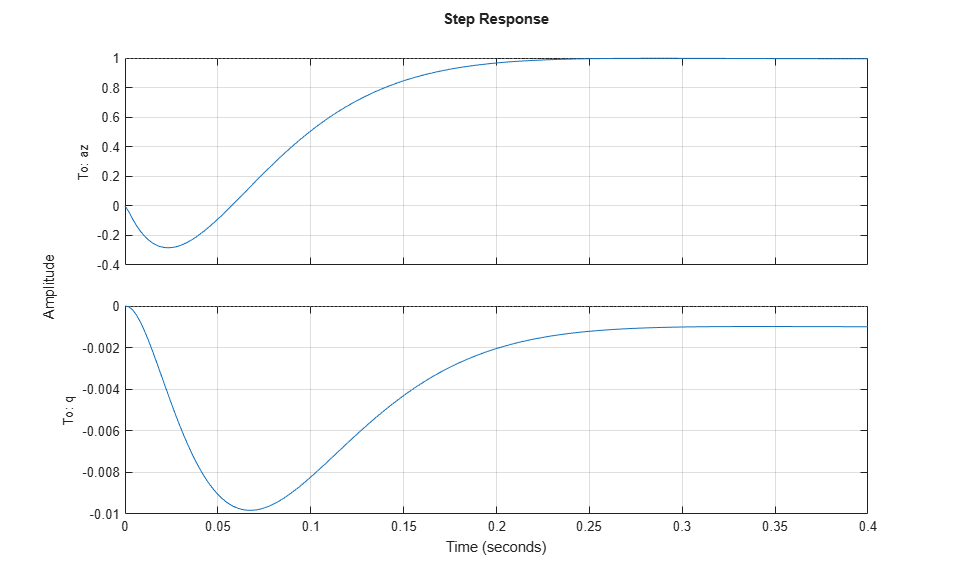
Plot the closed-loop response.
CL = feedback(G*Knom,diag([1 -1]));
step(CL(:,1)), grid
Robustness Analysis
Compute the disk margins at the plant input and outputs. That the az loop uses negative feedback while the q loop uses positive feedback, so change the sign of the loop gain of the q loop before using diskmargin.
loopsgn = diag([1 -1]);
Examine the margins at the plant input.
DM = diskmargin(Knom*loopsgn*G)
DM =

  struct with fields:

           GainMargin: [0.3918 2.5524]
          PhaseMargin: [-47.2105 47.2105]
           DiskMargin: 0.8740
           LowerBound: 0.8740
           UpperBound: 0.8740
            Frequency: 28.8842
    WorstPerturbation: [1×1 ss]
For the margins at plant outputs, use the multiloop margin to account for simultaneous, independent variations in both output channels.
[~,MM] = diskmargin(loopsgn*G*Knom)
MM =

  struct with fields:

           GainMargin: [0.4994 2.0025]
          PhaseMargin: [-36.9262 36.9262]
           DiskMargin: 0.6678
           LowerBound: 0.6678
           UpperBound: 0.6691
            Frequency: 23.6845
    WorstPerturbation: [2×2 ss]
Finally, compute the margins against simultaneous variations at the plant input and outputs.
MMIO = diskmargin(loopsgn*G,Knom)
MMIO =

  struct with fields:

           GainMargin: [0.6866 1.4565]
          PhaseMargin: [-21.0565 21.0565]
           DiskMargin: 0.3717
           LowerBound: 0.3717
           UpperBound: 0.3725
            Frequency: 24.8030
    WorstPerturbation: [1×1 struct]
The disk-based gain and phase margins exceed 2 (6dB) and 35 degrees at the plant input and the plant outputs. Moreover, MMIO indicates that this feedback loop can withstand gain variations by a factor 1.45 or phase variations of 21 degrees affecting all plant inputs and outputs at once.
Next, investigate the impact of gain and phase uncertainty on performance. Use the umargin control design block to model a gain change factor of 1.4 (3dB) and phase change of 20 degrees in each feedback channel. Use getDGM to fit an uncertainty disk to these amounts of gain and phase change.
GM = 1.4;
PM = 20;
DGM = getDGM(GM,PM,'balanced');
ue = umargin('e',DGM);
uq = umargin('q',DGM);
Gunc = blkdiag(ue,uq)*G;
Gunc.OutputName = {'az','q'};
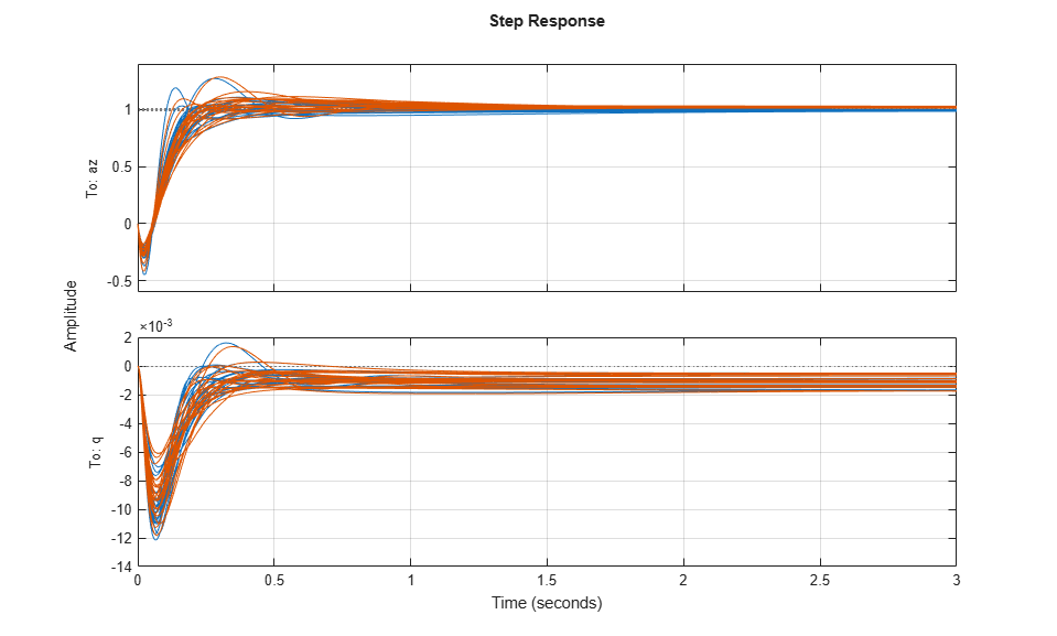
Rebuild the closed-loop model and sample the gain and phase uncertainty to gauge the impact on the step response.
CLunc = feedback(Gunc*Knom,loopsgn);
step(CLunc(:,1),3)
grid
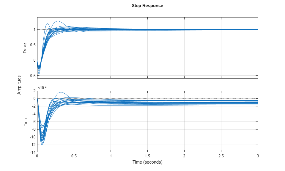
The plot shows significant variability in performance, with large overshoot and steady-state error for some combinations of gain and phase variations.
Robust Controller Synthesis
Redo the controller synthesis to account for gain and phase variations using musyn. This synthesis optimizes performance uniformly for the specified range of gain and phase uncertainty.
Punc = connect(Gunc,wS,wT,sb,{'azref','delta'},{'we','waz','e','q'});
[Kr,gam] = musyn(Punc,2,1);
gam
D-K ITERATION SUMMARY:
-----------------------------------------------------------------
                       Robust performance               Fit order
-----------------------------------------------------------------
  Iter         K Step       Peak MU       D Fit             D
    1           51.06        26.33        26.62             4
    2           7.028         5.24        5.304             8
    3           1.681        1.156        1.157             4
    4          0.9705       0.9702       0.9822            10
    5           0.962       0.9619       0.9622            10
    6          0.9625       0.9623       0.9629            10

Best achieved robust performance: 0.962


gam =

    0.9619
Compare the sampled step responses for the nominal and robust controllers. The robust design reduces both overshoot and steady-state errors and gives more consistent performance across the modeled range of gain and phase uncertainty.
CLr = feedback(Gunc*Kr,loopsgn);
rng(0) % for reproducibility
step(CLunc(:,1),3)
hold
rng(0)
step(CLr(:,1),3)
grid
Current plot held
The robust controller achieves this performance by increasing the (nominal) disk margins at the plant output and, to a lesser extent, the I/O disk margin. For instance, compare the disk-based margins at the plant outputs for the nominal and robust designs. Use diskmarginplot to see the variations of the margins with frequency.
Lnom = loopsgn*G*Knom;
Lrob = loopsgn*G*Kr;
clf
diskmarginplot(Lnom,Lrob)
title('Disk margins at plant outputs')
grid
legend('Nominal','Robust')

Examine the margins against variations simultaneous variations at the plant inputs and outputs with the robust controller.
MMIO = diskmargin(loopsgn*G,Kr)
MMIO =

  struct with fields:

           GainMargin: [0.6492 1.5404]
          PhaseMargin: [-24.0166 24.0166]
           DiskMargin: 0.4254
           LowerBound: 0.4254
           UpperBound: 0.4263
            Frequency: 19.6039
    WorstPerturbation: [1×1 struct]
Recall that with the nominal controller, the feedback loop could withstand gain variations of a factor of 1.45 or phase variations of 21 degrees affecting all plant inputs and outputs at once. With the robust controller, those margins increase to about 1.54 and 24 degrees.
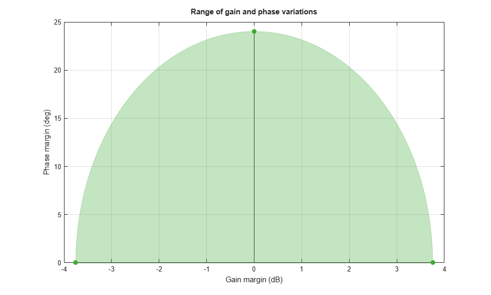
View the range of simultaneous gain and phase variations that the robust design can sustain at all plant inputs and outputs.
diskmarginplot(MMIO.GainMargin)
Nonlinear Simulation of Worst-Case Scenario
diskmargin returns the smallest change in gain and phase that destabilizes the feedback loop. It can be insightful to inject this perturbation in the nonlinear simulation to further analyze the implications for the real system. For example, compute the destabilizing perturbation at the plant outputs for the nominal controller.
[~,MM] = diskmargin(Lnom);
WP = MM.WorstPerturbation;
bode(WP)
title('Smallest destabilizing perturbation')
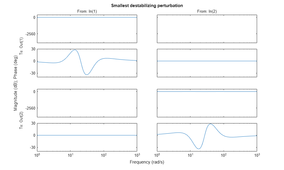
The worst perturbation is a diagonal, dynamic perturbation that multiplies the open-loop response at the plant outputs. With this perturbation, the closed-loop system becomes unstable with an undamped pole at the frequency w0 = MM.Frequency.
damp(feedback(WP*G*Knom,loopsgn))
         Pole              Damping       Frequency      Time Constant
                                       (rad/seconds)      (seconds)

 -1.88e-03                 1.00e+00       1.88e-03         5.33e+02
 -2.55e-02                 1.00e+00       2.55e-02         3.92e+01
 -3.20e-02                 1.00e+00       3.20e-02         3.12e+01
 -5.16e-02                 1.00e+00       5.16e-02         1.94e+01
 -1.25e-01                 1.00e+00       1.25e-01         7.98e+00
 -3.85e+00 + 5.04e+00i     6.07e-01       6.34e+00         2.60e-01
 -3.85e+00 - 5.04e+00i     6.07e-01       6.34e+00         2.60e-01
 -8.38e+00 + 1.17e+01i     5.81e-01       1.44e+01         1.19e-01
 -8.38e+00 - 1.17e+01i     5.81e-01       1.44e+01         1.19e-01
  4.49e-14 + 2.37e+01i    -1.89e-15       2.37e+01        -2.23e+13
  4.49e-14 - 2.37e+01i    -1.89e-15       2.37e+01        -2.23e+13
 -2.95e+01                 1.00e+00       2.95e+01         3.39e-02
 -3.33e+01                 1.00e+00       3.33e+01         3.00e-02
 -6.04e+01 + 2.28e+01i     9.36e-01       6.46e+01         1.66e-02
 -6.04e+01 - 2.28e+01i     9.36e-01       6.46e+01         1.66e-02
 -3.86e+01 + 5.36e+01i     5.85e-01       6.61e+01         2.59e-02
 -3.86e+01 - 5.36e+01i     5.85e-01       6.61e+01         2.59e-02
 -1.10e+03                 1.00e+00       1.10e+03         9.05e-04
w0 = MM.Frequency
w0 =

   23.6845
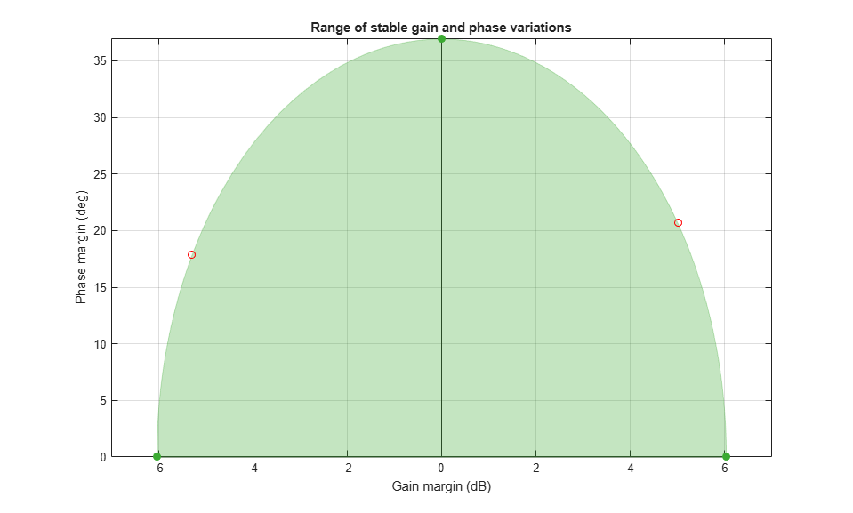
Note that the gain and phase variations induced by this perturbation lie on the boundary of the range of safe gain/phase variations computed by diskmargin. To confirm this result, compute the frequency response of the worst perturbation at the frequency w0, convert it to a gain and phase variation, and visualize it along with the range of safe gain and phase variations represented by the multiloop disk margin.
DELTA = freqresp(WP,w0);
clf
diskmarginplot(MM.GainMargin)
title('Range of stable gain and phase variations')
hold on
plot(20*log10(abs(DELTA(1,1))),abs( angle(DELTA(1,1))*180/pi),'ro')
plot(20*log10(abs(DELTA(2,2))),abs( angle(DELTA(2,2))*180/pi),'ro')
To simulate the effect of this worst perturbation on the full nonlinear model in Simulink, insert it as a block before the controller block, as done in the modified model rct_airframeWP.
close(f)
open_system('rct_airframeWP')
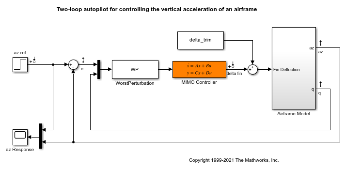
Here the MIMO Controller block is set to the nominal controller Knom. To simulate the nonlinear response with this controller, compute the trim deflection and q initial value from the operating condition op.
delta_trim = op.Inputs.u + [1.5 0]*op.States(5).x;
q_ini = op.States(4).x;
By commenting the WorstPerturbation block in and out, you can simulate the response with or without this perturbation. The results are shown below and confirm the destabilizing effect of the gain and phase variation computed by diskmargin.
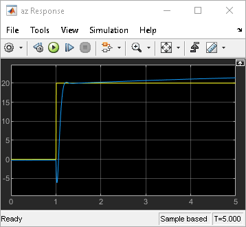
Figure 1: Nominal response.
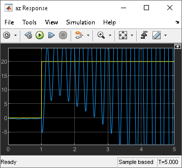
Figure 2: Response with destabilizing gain/phase perturbation.
See Also
umargin | diskmargin | diskmarginplot | musyn