Robust Vibration Control in Flexible Beam

This example shows how to robustly tune a controller for reducing vibrations in a flexible beam. This example is adapted from "Control System Design" by G. Goodwin, S. Graebe, and M. Salgado.

Uncertain Model of Flexible Beam

Figure 1 depicts an active vibration control system for a flexible beam.

Figure 1: Active control of flexible beam

In this setup, a sensor measures the tip position $$y(t)$$ and the actuator is a piezoelectric patch delivering a force $$u(t)$$. We can model the transfer function from control input $$u$$ to tip position $$y$$ using finite-element analysis. Keeping only the first six modes, we obtain a plant model of the form

$$G(s)=\sum _{i=1}^6\frac{{\alpha }_i}{s^2+2{\zeta }_i{\omega }_{i}s+{\omega }_i^2}$$

with the following nominal values for the amplitudes $${\alpha }_i$$ and natural frequencies $${\omega }_i$$:

$$\alpha =9.72\times 10^{-4},0.0122,0.0012,-0.0583,-0.0013,0.1199$$

$$\omega =18.95,118.76,332.54,651.66,1077.2,1609.2.$$

The damping factors $${\zeta }_i$$ are often poorly known and are assumed to range between 0.0002 and 0.02. Similarly, the natural frequencies are only approximately known and we assume 20% uncertainty on their location. To construct an uncertain model of the flexible beam, use the ureal object to specify the uncertainty range for the damping and natural frequencies. To simplify, we assume that all modes have the same damping factor $$\zeta$$.

% Damping factor
zeta = ureal('zeta',0.002,'Range',[0.0002,0.02]);

% Natural frequencies
w1 = ureal('w1',18.95,'Percent',20);
w2 = ureal('w2',118.76,'Percent',20);
w3 = ureal('w3',332.54,'Percent',20);
w4 = ureal('w4',651.66,'Percent',20);
w5 = ureal('w5',1077.2,'Percent',20);
w6 = ureal('w6',1609.2,'Percent',20);

Next combine these uncertain coefficients into the expression for $$G(s)$$.

alpha = [9.72e-4 0.0122 0.0012 -0.0583 -0.0013 0.1199];
G = tf(alpha(1),[1 2*zeta*w1 w1^2]) + tf(alpha(2),[1 2*zeta*w2 w2^2]) + ...
    tf(alpha(3),[1 2*zeta*w3 w3^2]) + tf(alpha(4),[1 2*zeta*w4 w4^2]) + ...
    tf(alpha(5),[1 2*zeta*w5 w5^2]) + tf(alpha(6),[1 2*zeta*w6 w6^2]);
G.InputName = 'uG';  G.OutputName = 'y';

Visualize the impact of uncertainty on the transfer function from $$u$$ to $$y$$. The bode function automatically shows the responses for 20 randomly selected values of the uncertain parameters.

rng(0), bode(G,{1e0,1e4}), grid
title('Uncertain beam model')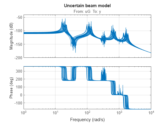

Robust LQG Control

LQG control is a natural formulation for active vibration control. With systune, you are not limited to a full-order optimal LQG controller and can tune controllers of any order. Here, for example, let's tune a 6th-order state-space controller (half the plant order).

C = tunableSS('C',6,1,1);

The LQG control setup is depicted in Figure 2. The signals $$d$$ and $$n$$ are the process and measurement noise, respectively.

Figure 2: LQG control structure

Build a closed-loop model of the block diagram in Figure 2.

C.InputName = 'yn';  C.OutputName = 'u';
S1 = sumblk('yn = y + n');
S2 = sumblk('uG = u + d');
CL0 = connect(G,C,S1,S2,{'d','n'},{'y','u'});

Note that CL0 depends on both the tunable controller C and the uncertain damping and natural frequencies.

CL0

Generalized continuous-time state-space model with 2 outputs, 2 inputs, 18 states, and the following blocks:
  C: Tunable 1x1 state-space model, 6 states, 1 occurrences.
  w1: Uncertain real, nominal = 18.9, variability = [-20,20]%, 3 occurrences
  w2: Uncertain real, nominal = 119, variability = [-20,20]%, 3 occurrences
  w3: Uncertain real, nominal = 333, variability = [-20,20]%, 3 occurrences
  w4: Uncertain real, nominal = 652, variability = [-20,20]%, 3 occurrences
  w5: Uncertain real, nominal = 1.08e+03, variability = [-20,20]%, 3 occurrences
  w6: Uncertain real, nominal = 1.61e+03, variability = [-20,20]%, 3 occurrences
  zeta: Uncertain real, nominal = 0.002, range = [0.0002,0.02], 6 occurrences

Type "ss(CL0)" to see the current value and "CL0.Blocks" to interact with the blocks.

Use an LQG criterion as control objective. This tuning goal lets you specify the noise covariances and the weights on the performance variables.

R = TuningGoal.LQG({'d','n'},{'y','u'},diag([1,1e-10]),diag([1 1e-12]));

Now tune the controller C to minimize the LQG cost over the entire uncertainty range.

[CL,fSoft,~,Info] = systune(CL0,R);

Soft: [5.63e-05,Inf], Hard: [-Inf,Inf], Iterations = 100
Soft: [6.27e-05,0.000102], Hard: [-Inf,-Inf], Iterations = 84
Soft: [6.96e-05,7.39e-05], Hard: [-Inf,-Inf], Iterations = 84
Soft: [7.19e-05,7.19e-05], Hard: [-Inf,-Inf], Iterations = 37
Final: Soft = 7.19e-05, Hard = -Inf, Iterations = 305

Validation

Compare the open- and closed-loop Bode responses from $$d$$ to $$y$$ for 20 randomly chosen values of the uncertain parameters. Note how the controller clips the first three peaks in the Bode response.

Tdy = getIOTransfer(CL,'d','y');
bode(G,Tdy,{1e0,1e4})
title('Transfer from disturbance to tip position')
legend('Open loop','Closed loop')

Next plot the open- and closed-loop responses to an impulse disturbance $$d$$. For readability, the open-loop response is plotted only for the nominal plant.

impulse(getNominal(G),Tdy,5)
title('Response to impulse disturbance d')
legend('Open loop','Closed loop')

Finally, systune also provides insight into the worst-case combinations of damping and natural frequency values. This information is available in the output argument Info.

WCU = Info.wcPert

WCU=3×1 struct array with fields:
    w1
    w2
    w3
    w4
    w5
    w6
    zeta

Use this data to plot the impulse response for the two worst-case scenarios.

impulse(usubs(Tdy,WCU),5)
title('Worst-case response to impulse disturbance d')

Related Examples

• Build Tunable Control System Model with Uncertain Parameters
• Robust Tuning of DC Motor Controller
• Robust Tuning of Mass-Spring-Damper System

More About

• Interpreting Results of Robust Tuning