Loop-Shaping Controller Design
This example shows how to design a controller by specifying a desired shape for the open-loop response of the plant with the controller. The loopsyn command designs a controller that shapes the open-loop response to approximately match the target loop shape you provide. loopsyn lets you adjust the tradeoff between performance and robustness to obtain satisfactory time-domain responses while avoiding fragile designs with plant inversion or flexible mode cancellation.
In this example, you design a controller for an aircraft model. The example shows how varying the balance between performance and robustness affects loop shape and closed-loop response. The example then shows how to reduce the controller order while preserving desirable characteristics of the response.
Plant Model
This example uses the two-input, two-output NASA HiMAT aircraft model [1]. The aircraft is shown in the following diagram.

The control variables are the elevon and canard actuators ( and ). The output variables are the angle of attack () and attitude angle (). The model has six states, given by
,
where and are the elevator and canard actuator states, respectively. Using the following state-space matrices, create a model of this plant.
A = [ -2.2567e-02  -3.6617e+01  -1.8897e+01  -3.2090e+01   3.2509e+00  -7.6257e-01;
       9.2572e-05  -1.8997e+00   9.8312e-01  -7.2562e-04  -1.7080e-01  -4.9652e-03;
       1.2338e-02   1.1720e+01  -2.6316e+00   8.7582e-04  -3.1604e+01   2.2396e+01;
       0            0            1.0000e+00   0            0            0;
       0            0            0            0           -3.0000e+01   0;
       0            0            0            0            0           -3.0000e+01];
B = [0     0;
     0     0;
     0     0;
     0     0;
    30     0;
     0    30];
C = [0     1     0     0     0     0;
     0     0     0     1     0     0];
D = [0     0;
     0     0];

G = ss(A,B,C,D);
G.InputName = {'elevon','canard'};
G.OutputName = {'attack','attitude'};
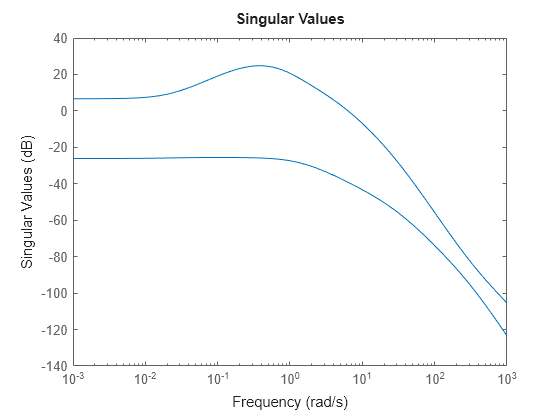
Examine the singular values of the model.
sigma(G)
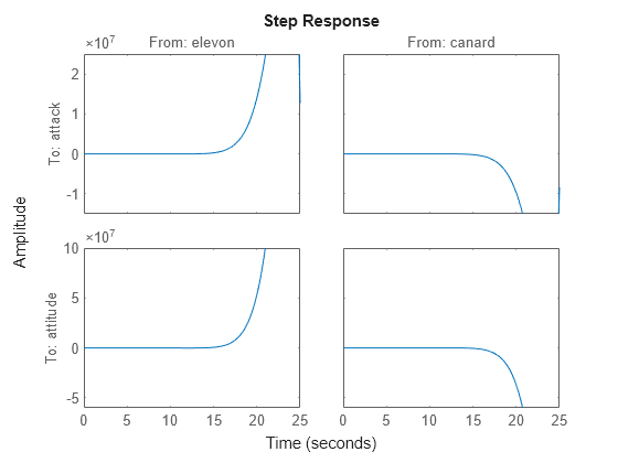
This plant is ill-conditioned, in the sense that it has a gap of about 40 dB between the largest and smallest singular values in the vicinity of the desired control bandwidth of 8 rad/s. Further, as a step plot shows, the open-loop response of this plant is unstable.
step(G)
Initial Controller Design
To design a stabilizing controller for this plant, select a target loop shape. A typical loop shape has low gain at high frequencies for robustness, and high gain at low frequencies for performance. For the desired crossover frequency of 8 rad/s, a simple target loop shape that meets these requirements is .
Gd = tf(8,[1 0]);
sigma(Gd,{0.1 100})
grid on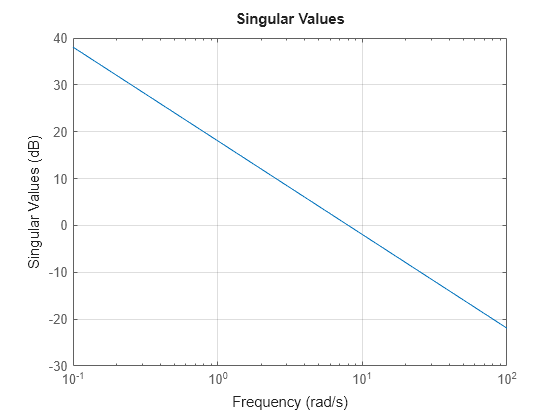
Design the initial controller with loopsyn.
[K0,CL0,gamma0,info0] = loopsyn(G,Gd);
gamma0
gamma0 =
1.2849
The performance gamma is a measure of how well the loop shape with K0 matches the desired loop shape. Values near or below 1 indicate that G*K0 is close to Gd. Compare the achieved loop shape with the target.
L0 = G*K0;
sigma(L0,"b",Gd,"r--",{.1,100});
grid
legend("L0 (actual loop shape)","Gd (target loop shape)");

The match is not very close at low frequencies, though it improves near crossover. Moreover, the two singular values are still somewhat far apart around crossover, such that the system has effectively two crossover frequencies. Examine how this open-loop shape affects the closed-loop step response.
step(CL0,5)
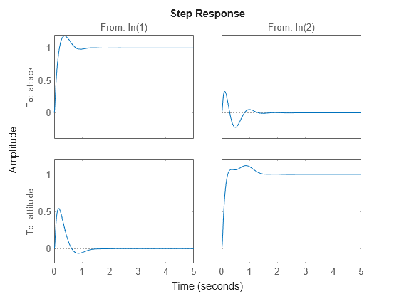
The bump in attitude tracking (lower-right plot) is the result of the separation of the two singular values, leading to a response with two time constants. Also, the response shows significant coupling between attack and attitude. You can adjust the controller to reduce the bump in attitude tracking, reduce the coupling, and if possible reduce the overshoot in the attack response.
Design Controller for Performance
To improve the design, you can try changing the balance that loopsyn strikes between performance and robustness. To do so, use the alpha input argument to loopsyn. By default, loopsyn uses alpha = 0.5, which optimizes performance subject to the robustness being no worse than half the maximum achievable robustness. alpha = 0 optimizes for performance (mixsyn design). Setting alpha = 1 uses the robustness-maximizing ncfsyn design. First, consider the pure mixsyn design.
alpha = 0;
[K_mix,CL_mix,gamma_mix,info_mix] = loopsyn(G,Gd,alpha);
gamma_mix
gamma_mix =
0.7723
The gamma value indicates a much closer match to the target loop shape, which you can confirm by plotting the open-loop responses.
L_mix = G*K_mix;
sigma(L0,"b",L_mix,"g",Gd,"r--",{.1,100});
grid
legend("L0 (initial design)","L_mix (mixsyn design)","Gd (target loop shape)");
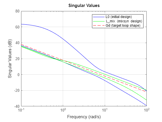
This design roughly inverts the plant. As a result, the singular values of L_mix converge near the crossover frequency and are generally much closer together than in the original plant. With this plant-inverting controller, the closed-loop response shows good performance, with minimal overshoot and cross-coupling.
step(CL0,CL_mix,5)
legend("Initial design","mixsyn design","Location","southeast")
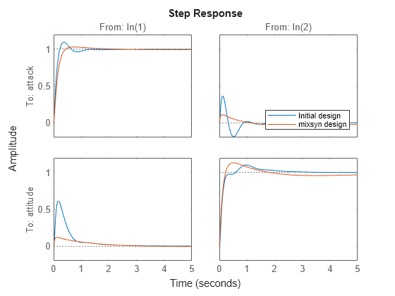
However, this performance comes at the cost of robustness. Compare the stability margins of the system with the initial design and the mixsyn design.
DM0 = diskmargin(G,K0);
DM_mix = diskmargin(G,K_mix);
DM0.DiskMargin
ans =
0.1192
DM_mix.DiskMargin
ans =
0.0517
The plant-inverting design has poor robustness. For instance, if the smallest singular value of the plant model is 1% of the largest singular value, inverting the plant amplifies model errors by a factor of 100 in the direction of the smallest singular value. Thus, unless you have a highly accurate model, use a design with better robustness.
Design Controller for Robustness
At the opposite extreme is the pure ncfsyn design, optimized for robustness. Compute such a controller using alpha = 1, and examine the resulting stability, loop shape, and responses.
alpha = 1;
[K_ncf,CL_ncf,gamma_ncf,info_ncf] = loopsyn(G,Gd,alpha);
gamma_ncf
gamma_ncf =
2.8360
DM_ncf = diskmargin(G,K_ncf);
DM_ncf.DiskMargin
ans =
0.2201
L_ncf = G*K_ncf;
sigma(L0,L_mix,L_ncf,Gd,"k--",{.1,100});
grid
legend("L0 (initial design)","L_mix (mixsyn design)",...
    "L_ncf (ncfsyn design)","Gd (target loop shape)");

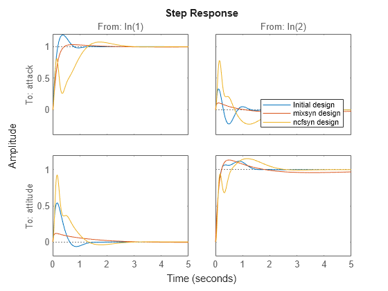
The increased value of gamma indicates poor performance, though the stability margin is improved, as expected. The singular-value plot shows that this controller inverts the plant even less than the initial design, which is evident in that the separation of the singular values is roughly the same as for the open-loop plant. The separation of crossover frequencies results in slow and fast time constants in the step response, which is even poorer than the initial design. The kick resulting from the wide crossover region is now apparent in all four I/O channels.
step(CL0,CL_mix,CL_ncf,5)
legend("Initial design","mixsyn design","ncfsyn design","Location","southeast")
Choosing a Satisfactory Design
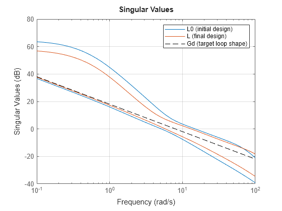
Thus, to improve on the default design, slightly favoring the mixsyn design without throwing away too much stability margin might yield a suitable design for this plant. You can control how much loopsyn favors performance or robustness by setting alpha to any value between 0 and 1. The default value used in the initial controller is alpha = 0.5. Try a value that slightly favors performance, and compare the results with the initial design.
alpha = 0.25;
[K,CL,gamma,info] = loopsyn(G,Gd,alpha);
gamma
gamma =
1.0114
L = G*K;
sigma(L0,L,Gd,"k--",{.1,100});
grid
legend("L0 (initial design)","L (final design)","Gd (target loop shape)");
DM = diskmargin(G,K);
DM.DiskMargin
ans =
0.0928
step(CL0,CL,5)
legend("initial (alpha = 0.5)","final (alpha = 0.25)","Location","southeast")
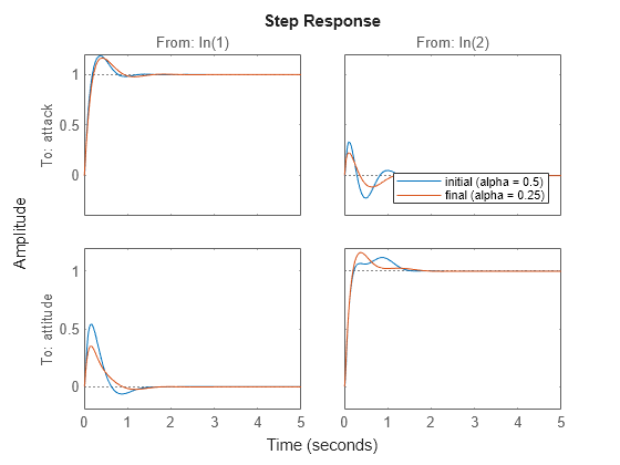
The alpha = 0.25 design yields reasonably good performance, reducing coupling and eliminating the bump in the attitude response. It has a slightly smaller stability margin (disk margin of about 0.09, compared to about 0.125 for the initial design). For your application, you can select whatever value of alpha between 0 and 1 achieves an acceptable balance between performance and robustness.
Conclusion
In conclusion, loopsyn lets you adjust the tradeoff between performance and robustness to strike a suitable balance for your application. You can try different values of alpha to find a controller that works for your requirements.
In some cases, you might want to find a suitable controller of lower order than that returned by loopsyn. One option is to use balred to reduce the controller order. However, reducing the controller in this way can change the balance of performance and robustness. To best preserve the desired performance and robustness characteristics, call loopsyn again using the ord input argument to directly synthesize a lower-order controller. Use the balred result to guide your choice of value for ord.
References
[1] Safonov, M., A. Laub, and G. Hartmann. “Feedback Properties of Multivariable Systems: The Role and Use of the Return Difference Matrix.” IEEE Transactions on Automatic Control 26, no. 1 (February 1981): 47–65.