Monopulse Comparator For Tracking Application using Rat race Couplers at X-band

Introduction:

This example shows how to implement a monopulse comparator using a rat-race coupler for tracking applications.

This comparator is designed over the X band frequencies and the simulated and measured results are compared.This guide is structured to assist users in building a comprehensive understanding of creating and analyzing RF PCBs in MATLAB, making it suitable for both beginners and experienced users.

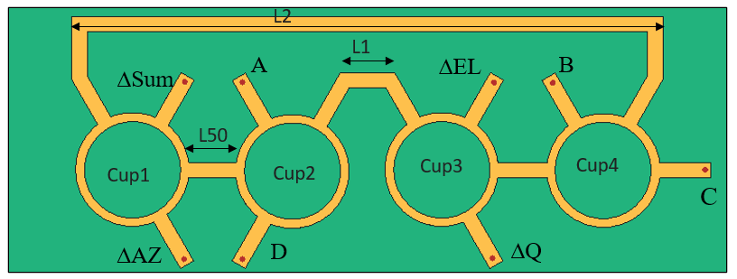
This diagram shows the top view of the antenna.

Create monopulse comparator

Design Parameters:

Start by setting the design parameters. These include dimensions for the couplers, line lengths, and the substrate properties. Adjust these parameters to fit your specific design requirements.

L1 = 5.56e-3;          % Branch Length in meters
L2 = 61e-3;            % Branch Length in meters
w50 = 1.565e-3;        % Width of 50 Ohm line in meters
L50 = 5.474e-3;        % Length of 50 Ohm line in meters
Rin = 4.97e-3;         % Inner Radius of Coupler in meters
RWidth = 0.9e-3;       % Width of the Ring in meters
Height = 0.508e-3;     % Height of the substrate in meters

Create First Ratrace Coupler:

Create Ring structure of ratrace coupler using ringAnnular object. Create port lines of ratrace coupler using antenna.Rectangle function.

% Creating Ring shape of first coupler -----------------
Ring = ringAnnular(Center=[-0.0230,0],InnerRadius=Rin,Width=RWidth);
% ------------------------Port 1 of first coupler----------------------------

p1 = antenna.Rectangle(Center=[-0.0314,0],Length=L50,Width=w50);
p1 = rotate(p1,180,[p1.Center,-1],[p1.Center,1]);
% ------------------------Port 2 of first coupler--------------------
p2 = antenna.Rectangle(Center=[-0.0188,0.0073],Length=L50,Width=w50);
p2 = rotate(p2,60,[p2.Center,-1],[p2.Center,1]);
% ------------------------Port 3 of first coupler--------------------
p3 = antenna.Rectangle(Center=[-0.0145,0],Length=L50,Width=w50);
p3 = rotate(p3,180,[p3.Center,-1],[p3.Center,1]);
% ------------------------Port 4 of first coupler--------------------
p4 = antenna.Rectangle(Center=[-0.0271,0.0074],Length=L50,Width=w50);
p4 = rotate(p4,-60,[p4.Center,-1],[p4.Center,1]);

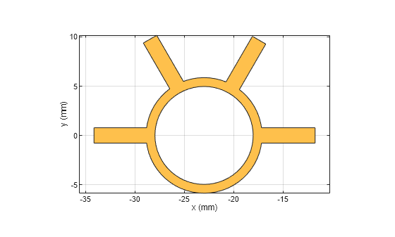
Create first coupler by adding all the shapes.

Cup1 = p1 + p2 + p3 + p4 + Ring;
show(Cup1)

Copy the shape to reuse.

copyCoupler1 = Cup1;

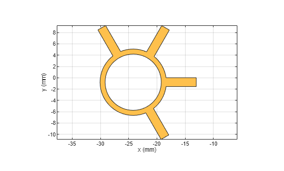
Use rotateZ and translate functions to rotate the coupler to fit in to the layout.

Cup1 = rotateZ(Cup1,-60);
Cup1 = translate(Cup1,[ -0.0127,-0.0207,0]);
show(Cup1)

Create other couplers by reusing first coupler

% *************** Making a copy of first coupler and rotating it to create the second coupler ***************
Cup2 = copy(copyCoupler1);
a2cen = [-0.0205,0.0197,0];
Cup2 = rotateZ(Cup2,120);
Cup2 = translate(Cup2,a2cen);
% *************** Making a copy of first coupler and rotating it to create the third coupler ***************
Cup3 = copy(Cup2);
Cup3 = mirrorY(Cup3);
% *************** Making a copy of first coupler and rotating it to create the fourth coupler ***************
Cup4 = copy(copyCoupler1);
a4cen = ([0.0129,0.0205,0]);
Cup4 = rotateZ(Cup4,60);
Cup4 = mirrorY(Cup4);
Cup4 = translate(Cup4,a4cen);

Create L1 shape

Use antenna.Rectangle to create L1 shape which connects cup2 and cup3.

% *************** Creating l1 shape ***************
L1Shape = antenna.Rectangle(Center=[0,0.0084],Length=L1,Width=w50);

Use tracePoint to create L2 shape which connects cup1 and cup4.

L2Shape = tracePoint;
L2Shape.TracePoints = [-30.5e-3+w50/2 8.43976e-3;-30.5e-3+w50/2 14.e-3;30.5e-3-w50/2 14.e-3;30.5e-3-w50/2 8.45e-3];
L2Shape.Width  = w50;

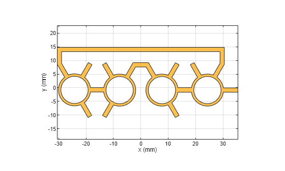
Add all the shapes to get toplayer.

Toplayer = Cup1 + Cup2 + Cup3 + Cup4 + L2Shape + L1Shape;
show(Toplayer)

Create PCB from Geometry

Use the pcbComponent object to create a PCB board assign the shape created in the previous section to the top layer of the pcb.

Comparator = pcbComponent;

Create board shape

% *************** Create board shape ***************
Ground = antenna.Rectangle(Center=[0 w50],Length=75e-3,Width=28e-3);
Comparator.BoardShape = Ground;
DielectricLayer = dielectric(EpsilonR=2.2,LossTangent=0,Thickness=Height);

Assign feed locations and layers.

feedloc = [[-0.0189,0.0083],[3 1];[-0.0190,-0.0100],[3 1];[-0.0129,0.0083],[3 1];[-0.0129,-0.0100],[3 1];
    [ 0.0131,0.0083],[3 1];[0.0129,-0.01],[3 1];[0.0191,0.0083],[3 1];[0.0349,-w50/2],[3 1]];
Comparator.FeedLocations = feedloc;
Comparator.FeedDiameter = 0.0005;
Comparator.BoardThickness = Height;
Comparator.Layers = {Toplayer,DielectricLayer,Ground};
show(Comparator);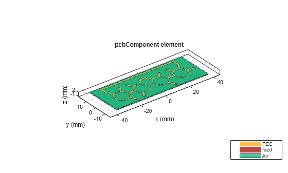

Analyze the device

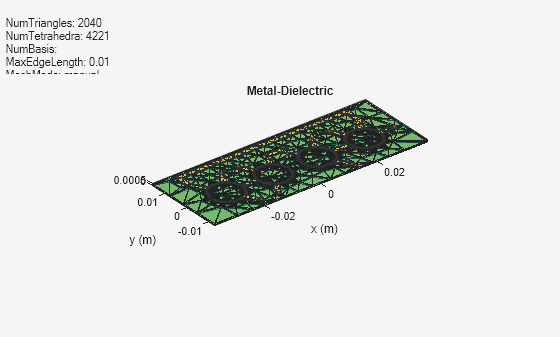
Creating the mesh

Manually mesh the PCB using the mesh function.

mesh(Comparator,maxEdgeLength=0.01);

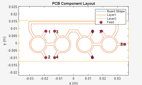
Use Layout method to see the port numbers for better understanding.

layout(Comparator)

Calculate S-Parameters

Calculate the S-parameters using the sparameters function.

spar=sparameters(Comparator,linspace(8e9,12e9,25));

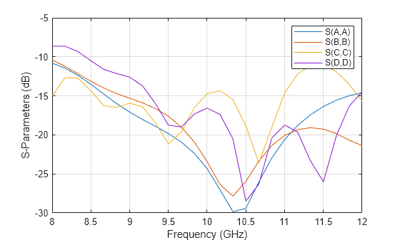
Plot S-parameters for 3, 4, 7, 8 ports considering them as A B C D respectively to get the monopulse comparator results.

figure;
rfplot(spar,3,3);
hold on;
rfplot(spar,4,4);
rfplot(spar,7,7);
rfplot(spar,8,8);
legend("S(A,A)","S(B,B)","S(C,C)","S(D,D)");
xlabel("Frequency (GHz)");
ylabel("S-Parameters (dB)");

Plot S-parameters for 3 to 1,2,5,6 ports considering them as SUM,AZ,EL,Q respectively to get the monopulse comparator results.

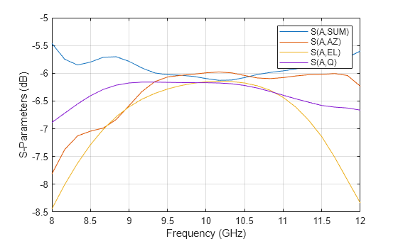
figure;
rfplot(spar,3,[1 2 5 6]);
legend("S(A,SUM)","S(A,AZ)","S(A,EL)","S(A,Q)");
xlabel("Frequency (GHz)");
ylabel("S-Parameters (dB)");

Plot S-parameters for 7 to 1,2,5,6 ports considering them as SUM,AZ,EL,Q respectively to get the monopulse comparator results.

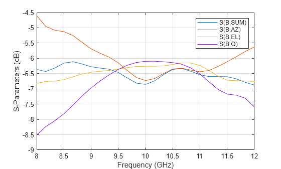
figure
rfplot(spar,7,[1 2 5 6]);
legend("S(B,SUM)","S(B,AZ)","S(B,EL)","S(B,Q)");
xlabel("Frequency (GHz)");
ylabel("S-Parameters (dB)");

Plot S-parameters for 8 to 1,2,5,6 ports considering them as SUM,AZ,EL,Q respectively to get the monopulse comparator results.

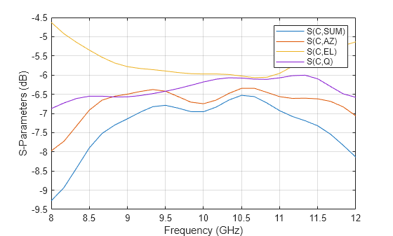
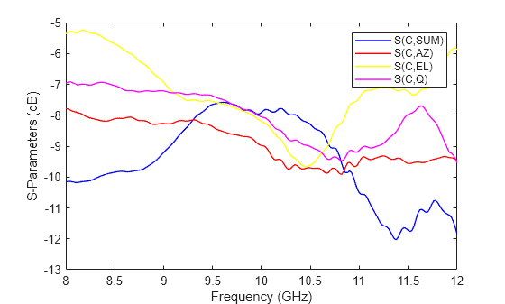
figure
rfplot(spar,8,[1 2 5 6]);
legend("S(C,SUM)","S(C,AZ)","S(C,EL)","S(C,Q)");
xlabel("Frequency (GHz)");
ylabel("S-Parameters (dB)");

Plot S-parameters for 4 to 1,2,5,6 ports considering them as SUM,AZ,EL,Q respectively to get the monopulse comparator results.

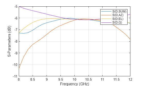
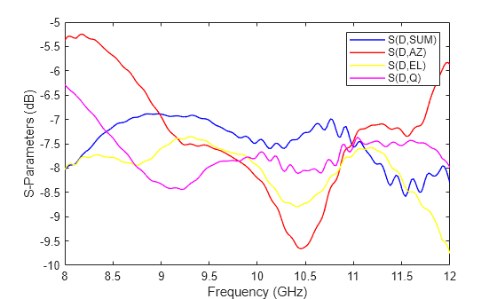
figure
rfplot(spar,4,[1 2 5 6]);
legend("S(D,SUM)","S(D,AZ)","S(D,EL)","S(D,Q)");
xlabel("Frequency (GHz)");
ylabel("S-Parameters (dB)");

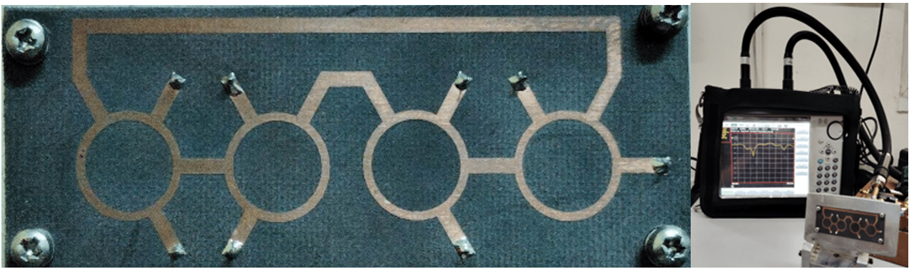
The designed monopulse comparator is fabricated as shown below and it is tested for the reflection coefficient at the sum and difference ports. Reflection coefficient of fabricated antenna array is measured using a Network Analyzer.

This figure shows the top view of the fabricated comparator and the measurement setup.

Measured Results

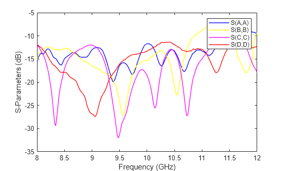
Plot the measured reflection coefficient.

load MonopulseData.mat
plot(Freq,AS11,"b",LineWidth=1);
hold on
plot(Freq,BS11,"Y",LineWidth=1);
plot(Freq,CS11,"m",LineWidth=1);
plot(Freq,DS11,"r",LineWidth=1);
hold off
xlabel("Frequency (GHz)");
ylabel("S-Parameters (dB)");
legend("S(A,A)","S(B,B)","S(C,C)","S(D,D)");

  %%
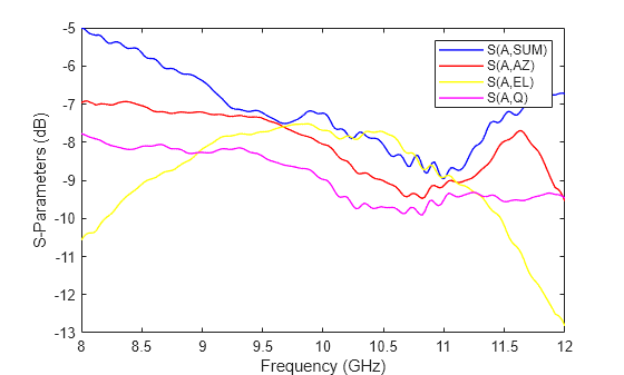
  plot(Freq,A_SUM,"b",LineWidth=1);  
  hold on
  plot(Freq,A_AZ,"r",LineWidth=1); 
  plot(Freq,A_EL,"Y",LineWidth=1);
  plot(Freq,A_Q,"m",LineWidth=1); 
  hold off
  xlabel("Frequency (GHz)");
  ylabel("S-Parameters (dB)");
  legend("S(A,SUM)","S(A,AZ)","S(A,EL)","S(A,Q)");

  %%
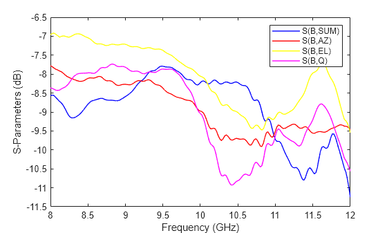
  plot(Freq,B_SUM,"b",LineWidth=1);
  hold on
  plot(Freq,B_AZ,"r",LineWidth=1);
  plot(Freq,B_EL,"Y",LineWidth=1);
  plot(Freq,B_Q,"m",LineWidth=1);  
  hold off
  xlabel("Frequency (GHz)");
  ylabel("S-Parameters (dB)");
  legend("S(B,SUM)","S(B,AZ)","S(B,EL)","S(B,Q)");

  %%
  plot(Freq,C_SUM,"b",LineWidth=1);
  hold on
  plot(Freq,C_AZ,"r",LineWidth=1);
  plot(Freq,C_EL,"Y",LineWidth=1);
  plot(Freq,C_Q,"m",LineWidth=1);  
  hold off
  xlabel("Frequency (GHz)");
  ylabel("S-Parameters (dB)");
  legend("S(C,SUM)","S(C,AZ)","S(C,EL)","S(C,Q)");

  %%
  plot(Freq,D_SUM,"b",LineWidth=1);
  hold on
  plot(Freq,D_AZ,"r",LineWidth=1);
  plot(Freq,D_EL,"Y",LineWidth=1);
  plot(Freq,D_Q,"m",LineWidth=1);  
  hold off
  xlabel("Frequency (GHz)");
  ylabel("S-Parameters (dB)");
  legend("S(D,SUM)","S(D,AZ)","S(D,EL)","S(D,Q)");

 %%
  
  

Conclusion:

The designed Monopulse comparator operats at X-band for tracking application . This design gives a good reflection coefficient below -10 dB, transmission coefficient close to -6 dB. The proposed comparator can serve as the main block in the mono-pulse antenna used for radar applications.