Simulate a Scanning Radar

This example shows how to simulate detection and tracking with a scanning monostatic radar. This example shows you how to configure a statistical radar model with mechanical and electronic scanning capabilities, how to set up a scenario management tool to handle platform dynamics and timing, and how to inspect the detections and tracks that are generated.

Introduction

Statistical Radar Model

Statistical radar models such as radarDataGenerator offer valuable data for early-stage development of radar systems. The system is modeled from the point of view of its performance characteristics, and a minimal set of parameters is used along with established theory to determine how this system will interact with its environment. This includes specification of fundamental system parameters such as operating frequency, bandwidth, and pulse repetition frequency (PRF), along with important metrics like angle and range resolution, false alarm rate, and detection probability. The radar model has dedicated modes for monostatic, bistatic, and passive operation. The primary output of this model is raw detection data or a sequence of track updates. While time-domain signals are not generated, an emitter can specify a numeric ID for the waveform it is using so that appropriate signal gain and rejection can be considered. Detections may be output in the radar frame, or in the scenario frame if the receiving radar has knowledge of the location and orientation of the transmitter. Tracks are generated using one of a variety of tracking and track management algorithms. Data rate is handled by a system update rate specification, so that detections are generated at the appropriate rate.

Scenario Management

The model works in tandem with a radarScenario to generate detection or track data over time in a dynamic environment. This scenario object not only manages the simulation time, but can handle the passing of data structures between objects in the scene as required when a frame of detection or track update is requested. The radar object is mounted on a platform which handles dynamics, such as position, velocity, and orientation in the scenario frame. These scenario platforms may also contain signature information, which describes how the platform appears to various types of sensors. For our purposes, the rcsSignature class will be used to endow target platforms with a radar cross section.

Scanning

Properties to control scanning can be found with the radar object definition. Scanning can be mechanical or electronic. With mechanical scanning, the pointing direction cannot change instantaneously, but is constrained by a maximum rotation rate in azimuth and elevation. With electronic scanning there is no such constraint, and the scan direction resets at the beginning of each loop. The radar is also allowed to perform mechanical and electronic scanning simultaneously.

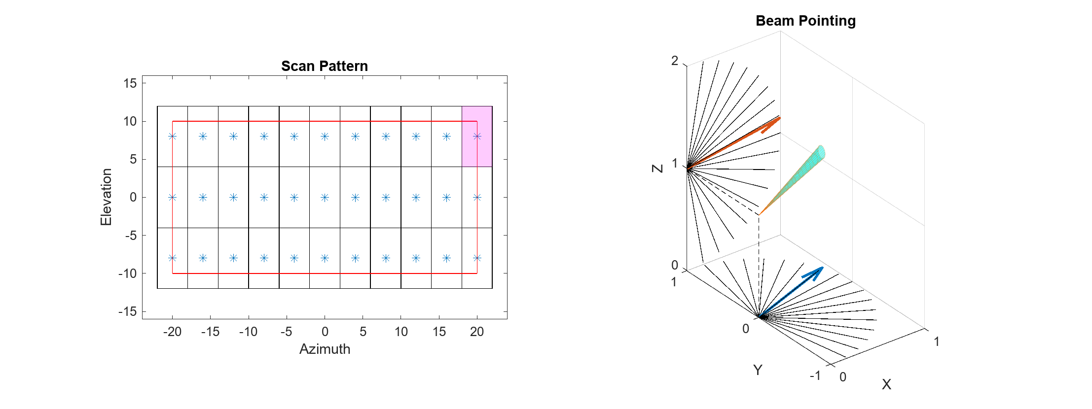
This figure shows the difference in scan pattern between these two modes. With the electronic mode the scan angle is always increasing, and with the mechanical mode the scan position always changes to an adjacent position. The radar scans in azimuth first because that is the primary scan direction, which is the direction with the greatest extent of the scan limit.

Scenario: Air Surveillance

For this scenario, consider a scanning radar system with its antenna mounted on a tower, as might be used for the tracking of aircraft. You will simulate a couple of inbound platforms with different RCS profiles, and inspect detection and track data. You can see the effect of SNR and range on the ability to make detections.

Radar System

Use a 1 GHz center frequency and a bandwidth of 1.5 MHz, to yield a range resolution of about 100 meters. To model a single pulse per scan position, set the update rate to the desired PRF. Set the size of the range ambiguity to reflect the PRF choice, and set the upper range limit to twice the size of the range ambiguity to enable detections of objects in the first and second range ambiguity.

% Set the seed for repeatability
rng('default');

% System parameters
c = physconst('lightspeed');
fc = 1e9; % Hz
bandwidth = 1.5e6; % Hz
prf = 4e3; % Hz
updateRate = prf;
rangeRes = c/(2*bandwidth); % m
rangeAmb = c/(2*prf); % m
rangeLims = [0 2*rangeAmb];

Besides choosing between mechanical and electronic scan modes, the scanning behavior is controlled by the specification of the scan limits and field of view (FoV) in azimuth and elevation. The FoV consists of the azimuth and elevation extent of the observable region at each scan position, similar to a two-sided half-power beamwidth specification. The scan points are chosen so that the total angular extent defined by the scan limit is covered by nonoverlapping segments with size equal to the FoV. Scan limits are specified in the radar's frame, which may be rotated from its platform's frame via the MountingAngles property.

Scan +/-20 degrees in azimuth and +/-10 degrees in elevation. Set the FoV to 4 degrees azimuth and 8 degrees elevation. Finally, specify the total number of complete scans to simulate, which will dictate the total simulation time.

% Scanning parameters
azLimits = [-20 20];
elLimits = [-10 10];
fov = [4;8]; % deg
numFullScans = 24; % number of full scans to simulate

The total number of scan points can be found as follows. The scan limits denote the minimum and maximum scan angles referenced to the antenna boresight vector, so the total area scanned in one direction is greater than the extent of the scan limits by up to half the FoV in that direction. The pattern is always a rectangular grid over az/el.

numScanPointsAz = floor(diff(azLimits)/fov(1)) + 1;
numScanPointsEl = floor(diff(elLimits)/fov(2)) + 1;
numScanPoints = numScanPointsAz*numScanPointsEl;

A specification of angular resolution separate from FoV is used, which allows for the modeling of angle estimation algorithms such as monopulse. This angular resolution determines the ability to discriminate between targets, and is used to derive the actual angle accuracy from the Cramer-Rao lower bound (CRLB) for monopulse angle estimation with that resolution. Similarly, range resolution determines the minimum spacing in range required to discriminate two targets, but the actual range measurement accuracy comes from the CRLB for range estimation. Exact measurables (range, range-rate, angle, etc.) can be used by turning measurement noise off with the HasNoise property. Typically, measurement error does not go to zero as SNR increases without bound. This can be captured by the bias properties (RangeBiasFraction, etc.), of which there is one for each type of measurable. For our purposes we will leave these at their defaults.

Use an angular resolution equal to 1/4th of the FoV in each direction, which allows discriminating between up to 16 point targets in the FoV at the same range.

angRes = fov/4;

Reference Target and Radar Loop Gain

Instead of directly specifying things like transmit power, noise power, and specifics of the detection algorithm used, this radar model uses the concept of radar loop gain to translate target RCS and range into an SNR, which is translated directly into a detection probability. Radar loop gain is an important property of any radar system, and is computed with a reference target, which consists of a reference range and RCS, and a receiver operating characteristic (ROC) for given detection and false alarm probabilities.

Use a detection probability of 90% for a reference target at 20 km and 0 dBsm. Use the default false alarm rate of 1e-6 false alarms per resolution cell per update.

refTgtRange = 20e3;
refTgtRCS = 0;
detProb = 0.9;
faRate = 1e-6;

Constructing the Radar

Construct the radar using the parameters above. Use the lower scan limit in elevation to set the pitch mounting angle of the radar from its platform. This points the boresight vector up so that the lower edge of the scanning area is parallel to the ground (that is, none of the scan points point the radar towards the ground).

pitch = elLimits(1); % mount the antenna rotated upwards

Enable elevation angle measurements, false alarm generation, and range ambiguities with the corresponding Has... property. To model a radar that only measures range and angle, set HasRangeRate to false. To get detections in scenario coordinates, the radar needs to be aware of the orientation of the transmitter. Because this example uses a monostatic radar, this can be achieved by enabling inertial navigation system (INS) functionality with the HasINS property.

% Create radar object
sensorIndex = 1; % a unique identifier is required
radar = radarDataGenerator(sensorIndex,'UpdateRate',updateRate,...
    'DetectionMode','Monostatic','ScanMode','Electronic','TargetReportFormat','Detections','DetectionCoordinates','scenario',...
    'HasElevation',true,'HasINS',true,'HasRangeRate',false,'HasRangeAmbiguities',true,'HasFalseAlarms',true,...
    'CenterFrequency',fc,'Bandwidth',bandwidth,...
    'RangeResolution',rangeRes,'AzimuthResolution',angRes(1),'ElevationResolution',angRes(2),...
    'ReferenceRange',refTgtRange,'ReferenceRCS',refTgtRCS,'DetectionProbability',detProb,'FalseAlarmRate',faRate,...
    'RangeLimits',rangeLims,'MaxUnambiguousRange',rangeAmb,'ElectronicAzimuthLimits',azLimits,'ElectronicElevationLimits',elLimits,...
    'FieldOfView',fov,'MountingAngles',[0 pitch 0]);

Use the helper class to visualize the scan pattern, and animate it in the simulation loop.

scanplt = helperScanPatternDisplay(radar);
scanplt.makeOverviewPlot;

The scan points in azimuth extend exactly to the specified azimuth scan limits, while the elevation scan points are pulled in slightly as needed to avoid overlapping or redundant scan points.

Calculate the total number of range-angle resolution cells for the system, and the total number of frames to be used for detection. Then compute the expected number of false alarms by multiplying the false alarm rate by the total number of resolution cells interrogated throughout the simulation.

numResolutionCells = diff(rangeLims)*prod(fov)/(rangeRes*prod(angRes));
numFrames = numFullScans*numScanPoints; % total number of frames for detection
expNumFAs = faRate*numFrames*numResolutionCells % expected number of FAs

expNumFAs = 9.5040

Scenario and Target

Use the radarScenario object to manage the top-level simulation flow. This object provides functionality to add new platforms and quickly generate detections from all sensor objects in the scenario. It also manages the flow of time in the simulation. Use the total number of frames calculated in the previous step to find the required StopTime. To adaptively update simulation time based on the update rate of objects in the scene, set the scenario update rate to zero.

% Create scenario
stopTime = numFullScans*numScanPoints/prf;
scene = radarScenario('StopTime',stopTime,'UpdateRate',0);

Use the platform method to generate new platform objects, add them to the scene, and return a handle for accessing the platform properties. Each platform has a unique ID, which is assigned by the scenario upon construction. For a static platform, only the Position property needs to be set. To simulate a standard constant-velocity kinematic trajectory, use the kinematicTrajectory object and specify the position and velocity.

Create two target platforms at different ranges, both inbound at different speeds and angles.

% Create platforms
rdrPlat = platform(scene,'Position',[0 0 12]); % place 12 m above the origin
tgtPlat(1) = platform(scene,'Trajectory',kinematicTrajectory('Position',[38e3 6e3 10e3],'Velocity',[-380 -50 0]));
tgtPlat(2) = platform(scene,'Trajectory',kinematicTrajectory('Position',[25e3 -3e3 1e3],'Velocity',[-280 10 -10]));

To enable convenience detection methods and automatic advancement of simulation time, the scenario needs to be aware of the radar object constructed earlier. To do this, mount the radar to the platform by populating the Sensors property of the platform. To mount more than one sensor on a platform, the Sensors property may be a cell array of sensor objects.

% Mount radar to platform
rdrPlat.Sensors = radar;

The rcsSignature class can be used to specify platform RCS as a function of aspect angle. For a simple constant-RCS signature, set the Pattern property to a scalar value. Let one platform be 20 dBsm and the other 4 dBsm to demonstrate the difference in detectability.

% Set target platform RCS profiles
tgtRCS = [20, 4]; % dBsm
tgtPlat(1).Signatures = rcsSignature('Pattern',tgtRCS(1));
tgtPlat(2).Signatures = rcsSignature('Pattern',tgtRCS(2));

Detectability

Calculate the theoretical SNR that can be expected for our targets. Because a simple kinematic trajectory is used, the truth position and range is calculated as such.

time = (0:numFrames-1).'/updateRate;
tgtPosTruth(:,:,1) = tgtPlat(1).Position + time*tgtPlat(1).Trajectory.Velocity;
tgtPosTruth(:,:,2) = tgtPlat(2).Position + time*tgtPlat(2).Trajectory.Velocity;
tgtRangeTruth(:,1) = sqrt(sum((tgtPosTruth(:,:,1)-rdrPlat.Position).^2,2));
tgtRangeTruth(:,2) = sqrt(sum((tgtPosTruth(:,:,2)-rdrPlat.Position).^2,2));

Then use the known target RCS and the radar loop gain computed by the radar model to get the truth SNR for each target.

tgtSnr = tgtRCS - 40*log10(tgtRangeTruth) + radar.RadarLoopGain;

For a magnitude-only detection scheme, such as CFAR, with the specified probability of detection and false alarm rate, the minimum SNR required for detection is given by

minSnr = 20*log10(erfcinv(2*radar.FalseAlarmRate) - erfcinv(2*radar.DetectionProbability)); % dB

Compute the minimum range for detection.

Rd = 10.^((tgtRCS - minSnr + radar.RadarLoopGain)/40); % meters

Compare the mean range and SNR of the targets to the minimum range and SNR thresholds. The total travel distance of the targets is small enough that the range-based SNR does not change significantly.

snrMargin = mean(tgtSnr,1) - minSnr

snrMargin = 1×2

    8.6781    0.5978

rangeMargin = (Rd - mean(tgtRangeTruth,1))/1e3 % km

rangeMargin = 1×2

   25.7310    0.8812

The first target is about 8 dB brighter than needed for detection with the given CFAR parameters, while the second target is considered barely detectable.

Simulate Detections

The primary simulation loop starts by calling advance on the scenario object. This method steps the scenario forward to the next time at which an object in the scene requires an update, and returns false when the specified stop time is reached, exiting the loop. Note that the first call to advance does not step the simulation time, so that the first frame of data collection may occur at 0 s. As an alternative to using advance, scene.SimulationStatus can be checked to determine if the simulation has run to completion.

Inside the loop, the detection and track generation methods can be called for any sensor object individually (see the sensor step method), but convenience methods exist to generate detections and tracks for all sensors and from all targets in the scene with one function call. Because we only have one sensor, detect(scene) is a good solution to get a list of detections for all targets in the scene. By initiating the generation of detections at the top level like this, the scene itself handles the passing of required timing, INS, and other configuration data to the sensor. The visualization helper class is used here as well to animate the scan pattern.

allDets = []; % initialize list of all detections generated
lookAngs = zeros(2,numFrames);
simTime = zeros(1,numFrames);
frame = 0; % current frame
while advance(scene) % advance until StopTime is reached
    
    % Increment frame index and record simulation time
    frame = frame + 1;
    simTime(frame) = scene.SimulationTime;
    
    % Generate new detections
    dets = detect(scene);
    
    % Record look angle for inspection
    lookAngs(:,frame) = radar.LookAngle;
    
    % Update coverage plot
    scanplt.updatePlot(radar.LookAngle);
    
    % Compile any new detections
    allDets = [allDets;dets];
    
end

Scan Behavior

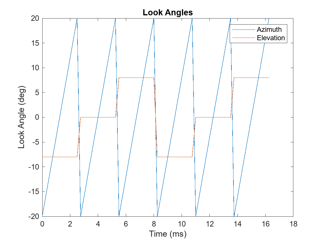
Plot the recorded look angles for the first two complete scans to inspect the pattern. The radar scans first in azimuth, and steps up in elevation at the end of each azimuth scan, instantaneously resetting the look angle at the start of each new scan.

figure;
plot(simTime(1:2*numScanPoints)*1e3,lookAngs(:,1:2*numScanPoints));
xlabel('Time (ms)');
ylabel('Look Angle (deg)');
legend('Azimuth','Elevation');
title('Look Angles');

Detections

Inspect the contents of an objectDetection as output by our radar.

allDets{1}

ans = 
  objectDetection with properties:

                     Time: 7.5000e-04
              Measurement: [3×1 double]
         MeasurementNoise: [3×3 double]
              SensorIndex: 1
            ObjectClassID: 0
    ObjectClassParameters: []
    MeasurementParameters: [1×1 struct]
         ObjectAttributes: {[1×1 struct]}

Time is the simulation time at which the radar generated the detection. SensorIndex shows which sensor this detection was generated by (which is important when there are multiple sensors and you are using the scene-level detect method). Measurement is the measurable value associated with the detection. The format depends on the choice of the detection mode and output coordinates. MeasurementNoise gives the variance or covariance of the measurement and is used by tracker models. When outputting detections in scenario coordinates, the measurement field is simply the estimated position vector of the target, and the measurement noise gives the covariance of that position estimate.

The ObjectAttributes field contains some useful metadata. Inspect the contents of the metadata for the first detection.

allDets{1}.ObjectAttributes{1}

ans = struct with fields:
    TargetIndex: 3
            SNR: 13.1821

TargetIndex shows the index of the platform that generated the detection, which is the unique identifier assigned by the scenario in the order the platforms are constructed. The SNR of this detection is about what we expected from the corresponding target platform. When the detection is a false alarm, TargetIndex will be -1, which is an invalid platform ID.

Collect the target index, SNR, and time of each detection into vectors.

detTgtIdx = cellfun(@(t) t.ObjectAttributes{1}.TargetIndex, allDets);
detTgtSnr = cellfun(@(t) t.ObjectAttributes{1}.SNR, allDets);
detTime   = cellfun(@(t) t.Time, allDets);
firstTgtDet  = find(detTgtIdx == tgtPlat(1).PlatformID);
secondTgtDet = find(detTgtIdx == tgtPlat(2).PlatformID);

Find the total number of FA detections.

numFAs = numel(find(detTgtIdx==-1))

numFAs = 9

This is close to the expected number of FAs computed earlier.

Collect the measurement data across detections and plot along with truth positions for the two target platforms.

tgtPosObs = cell2mat(cellfun(@(t) t.Measurement,allDets,'UniformOutput',0).');
subplot(1,2,1);
helperPlotPositionError( tgtPosTruth(:,:,1),time,tgtPosObs(:,firstTgtDet),detTime(firstTgtDet),scene.SimulationTime );
title('Target 1 Position Error');
subplot(1,2,2);
helperPlotPositionError( tgtPosTruth(:,:,2),time,tgtPosObs(:,secondTgtDet),detTime(secondTgtDet),scene.SimulationTime );
title('Target 2 Position Error');
set(gcf,'Position',get(gcf,'Position')+[0 0 600 0]);

Most of the detections originate from the first target. However, the first target was not detected on every frame, and the second target has generated many detections despite having a low SNR. Though the first target is easily detected, the measurement error is large because the target is in the second range ambiguity and no disambiguation has been performed. The second target, when detected, shows position error that is consistent with 100 meter range resolution and relatively-poor angle resolution.

Look at the total variance of the detections against SNR. The total variance is the sum of the marginal variances in each Cartesian direction (X, Y, and Z). This variance includes the effects of estimation in range-angle space along with the transformation of those statistics to scenario coordinates.

detTotVar = cellfun(@(t) trace(t.MeasurementNoise),allDets);
figure;
subplot(1,2,1);
helperPlotPositionTotVar( detTgtSnr(firstTgtDet),detTotVar(firstTgtDet) );
title('First Target');
subplot(1,2,2);
helperPlotPositionTotVar( detTgtSnr(secondTgtDet),detTotVar(secondTgtDet) );
title('Second Target');
set(gcf,'Position',get(gcf,'Position')+[0 0 600 0]);

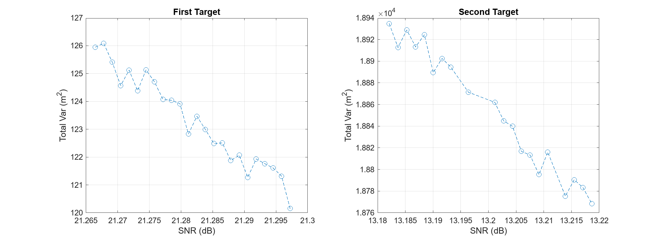
Although the absolute position error for the first target was greater due to the range ambiguity, the lower measurement variance reflects both the greater SNR of the first target and its apparently short range.

Simulate Tracks

The radarDataGenerator is also capable of performing open-loop tracking. Instead of outputting detections, it can output track updates.

Run the simulation again, but this time let configure the radar model to output tracks directly. Firstly, set some properties of the radar model to generate tracks in the scenario frame.

release(radar); % unlock for re-simulation
radar.TargetReportFormat = 'Tracks';
radar.TrackCoordinates = 'Scenario';

Tracking can be performed by a number of different algorithms. There are simple alpha-beta filters and Kalman filters of the linear, extended, and unscented variety, along with constant-velocity, constant-acceleration, and constant-turnrate motion models. Specify which algorithm to use with the FilterInitializationFcn property. This is a function handle or the name of a function in a character vector, for example @initcvekf or 'initcvekf'. If using a function handle, it must take an initial detection as input and return an initialized tracker object. Any user-defined function with the same signature may be used. For this example, use the constant-velocity extended Kalman filter.

radar.FilterInitializationFcn = @initcvekf;

The overall structure of the simulation loop is the same, but in this case the radar's step function must be called manually. The required inputs are a target poses structure, acquired by calling targetPoses on the radar platform, the INS structure, acquired by calling pose on the radar platform, and the current simulation time.

restart(scene); % restart scenario

allTracks = []; % initialize list of all track data
while advance(scene)
    
    % Generate new track data
    tgtPoses = targetPoses(rdrPlat);
    ins = pose(rdrPlat);
    tracks = radar(tgtPoses,ins,scene.SimulationTime);
    
    % Compile any new track data
    allTracks = [allTracks;tracks];
    
end

Inspect a track object.

allTracks(1) % look at first track update

ans = 
  objectTrack with properties:

                     TrackID: 1
                    BranchID: 0
                 SourceIndex: 1
                  UpdateTime: 0.0093
                         Age: 34
                       State: [6×1 double]
             StateCovariance: [6×6 double]
             StateParameters: [1×1 struct]
               ObjectClassID: 0
    ObjectClassProbabilities: 1
                  TrackLogic: 'History'
             TrackLogicState: [1 1 0 0 0]
                 IsConfirmed: 1
                   IsCoasted: 0
              IsSelfReported: 1
            ObjectAttributes: [1×1 struct]

TrackID is the unique identifier of the track file, and SourceIndex is the ID of the tracker object reporting the track, which is useful when you have multiple trackers in the scene. When a multi-hypothesis tracker is used, BranchID gives the index of the hypothesis used. The State field contains the state information on this update. Because a constant-velocity model and scenario-frame track coordinates are used, State consists of the position and velocity vectors. UpdateTime gives the time at which this track update was generated. Another important property, IsCoasted, tells you if this track update used a fresh target detection to update the filter, or if it was simply propagated forward in time from the last target detection (the track is "coasted").

The ObjectAttributes structure gives the ID of the platform whose signature is being detected, and the SNR of that signature during the update.

allTracks(1).ObjectAttributes

ans = struct with fields:
    TargetIndex: 3
            SNR: 19.1837

Collect the target index and update time. Also check how many detections were used to update our tracks.

trackTgtIdx = arrayfun(@(t) t.TargetIndex,[allTracks.ObjectAttributes]);
updateTime = [allTracks.UpdateTime];
firstTgtTrack = find(trackTgtIdx == tgtPlat(1).PlatformID);
secondTgtTrack = find(trackTgtIdx == tgtPlat(2).PlatformID);

numUpdates = numel(find(~[allTracks.IsCoasted])) % total number of track updates with new detection data

numUpdates = 33

This is roughly the number of non-FA detections generated in the first part.

Look at the reported positions in the XY plane and their covariances, along with truth position data. Because the first target is in the second range ambiguity and no disambiguation was performed, find the "truth" ambiguous position for the first target.

los = tgtPosTruth(:,:,1) - rdrPlat.Position;
R = sqrt(sum(los.^2,2));
los = los./R;
Ramb = mod(R,rangeAmb);
tgtPosTruthAmb = rdrPlat.Position + los.*Ramb;

Use the helper function to plot a visualization of the position track.

figure;
subplot(1,2,1);
helperPlotPositionTrack( tgtPosTruthAmb,allTracks(firstTgtTrack) );
title('First Target Track');
subplot(1,2,2);
helperPlotPositionTrack( tgtPosTruth(:,:,2),allTracks(secondTgtTrack) );
title('Second Target Track');
set(gcf,'Position',get(gcf,'Position')+[0 0 600 0]);

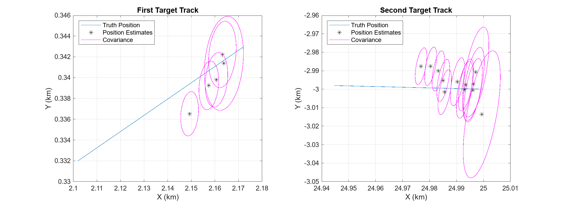
In both cases, the position estimates start by converging on the truth (or range-ambiguous truth) trajectory. For the first target we have more track updates and the final state appears closer to steady-state convergence. Looking at the covariance contours, notice the expected initial decrease in size as the tracking filter warms up.

To take a closer look at the tracking performance, plot the magnitude of the position estimation error for both targets, and indicate which samples were updated with target detections.

figure;
subplot(1,2,1);
helperPlotPositionTrackError( tgtPosTruthAmb,time,allTracks(firstTgtTrack),updateTime(firstTgtTrack) );
title('First Target Ambiguous Position Error');
subplot(1,2,2);
helperPlotPositionTrackError( tgtPosTruth(:,:,2),time,allTracks(secondTgtTrack),updateTime(secondTgtTrack) );
title('Second Target Position Error');
set(gcf,'Position',get(gcf,'Position')+[0 0 600 0]);

For the first target, which has a larger SNR, the position error decreases on samples that had a new detection to update the track file (indicated by a red circle). Since the second target had much lower SNR, the error in some individual detections was great enough to increase the position error of the track. Despite this, the second target track position error has an initial downward trend, and the estimated state will likely converge.

There is an issue with the first target track. Because it is in the second range ambiguity and has a component of motion perpendicular to the line of sight, the apparent velocity is changing, and the constant-velocity Kalman filter is unable to converge.

Conclusion

In this example you configured a statistical radar system for use in the simulation and analysis of target detectability and trackability. You saw how to use the scan limits and field of view properties to define a scan pattern, how to run the radar model with a scenario management tool, and how to inspect the generated detections and tracks.

Helper Functions

function helperPlotPositionError( tgtPosTruth,time,tgtPosObs,detTime,T )

tgtPosTruthX = interp1(time,tgtPosTruth(:,1),detTime).';
tgtPosTruthY = interp1(time,tgtPosTruth(:,2),detTime).';
tgtPosTruthZ = interp1(time,tgtPosTruth(:,3),detTime).';

err = sqrt((tgtPosTruthX - tgtPosObs(1,:)).^2+(tgtPosTruthY - tgtPosObs(2,:)).^2+(tgtPosTruthZ - tgtPosObs(3,:)).^2);

plot(detTime*1e3,err/1e3,'--o');
grid on;
xlim([0 T*1e3]);
ylabel('RMS Error (km)');
xlabel('Time (ms)');

end

function helperPlotPositionTotVar( detTgtSnr,detTotVar )

plot(detTgtSnr,detTotVar,'--o');
grid on;
xlabel('SNR (dB)');
ylabel('Total Var (m^2)');

end

function helperPlotPositionTrack( tgtPosTruth,tracks )

plot(tgtPosTruth(:,1)/1e3,tgtPosTruth(:,2)/1e3);
hold on;

updateIdx = find(~[tracks.IsCoasted]);
theta = 0:0.01:2*pi;

for ind = 1:2:numel(updateIdx)
    
    % plot update
    T = tracks(updateIdx(ind));
    plot(T.State(1)/1e3,T.State(3)/1e3,'*black');
    sigma = T.StateCovariance([1 3],[1 3]);
    [evec,eval] = eigs(sigma);
    mag = sqrt(diag(eval)).';
    u = evec(:,1)*mag(1);
    v = evec(:,2)*mag(2);
    x = cos(theta)*u(1) + sin(theta)*v(1);
    y = cos(theta)*u(2) + sin(theta)*v(2);
    plot(x/1e3 + T.State(1)/1e3,y/1e3 + T.State(3)/1e3,'magenta');
    
end

hold off;
grid on;
xlabel('X (km)');
ylabel('Y (km)');
legend('Truth Position','Position Estimates','Covariance','Location','northwest');

end

function helperPlotPositionTrackError( tgtPosTruth,time,tracks,updateTime )

state = [tracks.State];

sx = state(1,:);
sy = state(3,:);
sz = state(5,:);

x = interp1(time,tgtPosTruth(:,1),updateTime);
y = interp1(time,tgtPosTruth(:,2),updateTime);
z = interp1(time,tgtPosTruth(:,3),updateTime);

err = sqrt((x-sx).^2+(y-sy).^2+(z-sz).^2);

isUpdate = ~[tracks.IsCoasted];

plot(updateTime*1e3,err);
hold on;
plot(updateTime(isUpdate)*1e3,err(isUpdate),'or');
hold off;
grid on;
xlabel('Update Time (ms)');
ylabel('Error (m)')
legend('Coasted','Update','Location','northwest');

end