Nonlinear Features
Nonlinear features provide metrics that characterize chaotic behavior in vibration signals. These features can be useful in analyzing vibration and acoustic signals from systems such as bearings, gears, and engines. Nonlinear feature generation is more computationally intensive than the generation of any other features in the app.
The unique benefit of nonlinear features is that these features reflect changes in phase space trajectory of the underlying system dynamics. These changes can surface even before the occurrence of a fault condition. Thus, monitoring system dynamic characteristics using nonlinear features can help identify potential faults earlier, such as when a bearing is slightly worn.
Phase-Space Reconstruction Parameters
All the nonlinear features rely on phase-space reconstruction. Phase space is a multidimensional mapping of all possible variable states. This mapping provides a portrait of the fully dynamic behavior of a system. Phase-space reconstruction is a technique that recreates the multidimensional phase space from a single one-dimensional signal.
Embedding dimension — Dimension of the phase space, equivalent to the number of state variables in the dynamic system
Lag — Delay value used to perform the reconstruction
The default ‘Auto’ setting results in estimation of these
parameters. Vary the parameters manually to explore the impact of the settings on the
effectiveness of the resulting features.
For more information on phase-space reconstruction, see phaseSpaceReconstruction.
Approximate Entropy
Approximate entropy measures the regularity in the signal, or conversely, the signal unpredictability. Degradation within a system typically increases the approximate entropy.
Radius — Similarity criterion that identifies a meaningful range in which fluctuations in data are to be considered similar. The
‘Auto’setting invokes the default, which is based on the variance or covariance of the signal.
Correlation Dimension
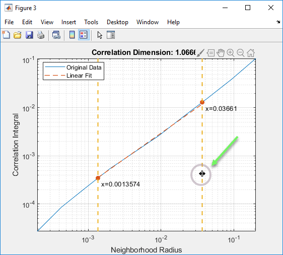
Correlation dimension measures chaotic signal complexity, which reflects self-similarity. Degradation typically increases signal complexity and in doing so increases the value of this metric.
Similarity radius — Bounding range for points to be included in the correlation dimension calculation. The default values are based on the signal covariance.
Explore radius values visually using Explore. Explore brings up a plot of correlation integral versus radius. The correlation integral is the mean probability that the states of a system are close at two different time intervals. This integral reflects self-similarity. You can modify the similarity range by moving either of the vertical bounding lines, as shown in the following figure. The goal is to bound a linear portion of the curve. The bounding values transfer automatically to the Correlation dimension settings when you close the figure.
Number of points — Number of points between the min and max range values. This setting drives the resolution of the calculation.
For more information on correlation dimension, see correlationDimension.
Lyapunov Exponent
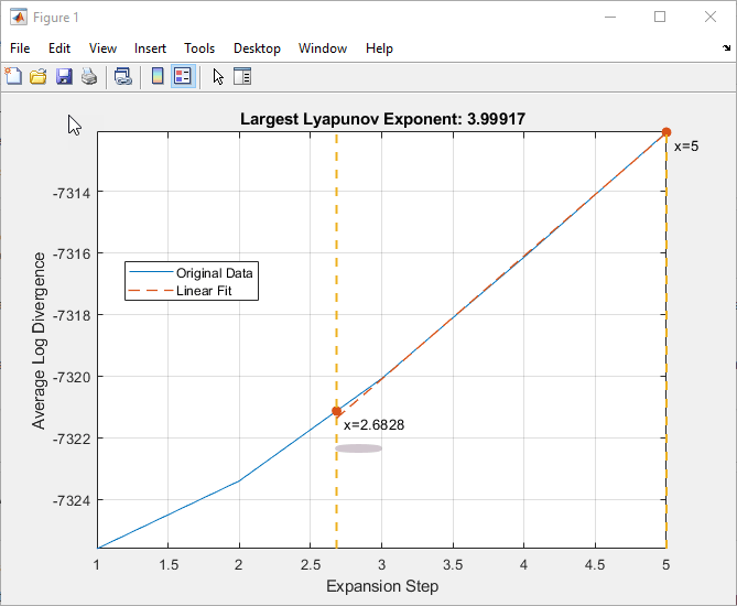
The Lyapunov exponent measures the degree of chaos due to signal abnormality, based on the rate of separation of infinitesimally close trajectories in phase space. Degradation within the system increases this value. A positive Lyapunov exponent indicates the presence of chaos, with degree related to the magnitude of the exponent. A negative exponent indicates a nonchaotic signal.
Expansion range – Bounding integer range that delimits the points to be used to estimate the local expansion rate. This rate is then used to calculate the Lyapunov exponent.
Explore the relationship between the expansion range and the expansion rate (average log divergence) visually by using Explore. Select a portion of the plot that is linear, using integers to bound the region. The bounding values transfer automatically to the Min and Max Expansion range settings when you close the figure.
Mean period — Threshold integer value used to find the nearest neighbor for a specific point to estimate the largest Lyapunov exponent. The software bases the default value on the mean frequency of the signal.
For more information on the Lyapunov exponent, see lyapunovExponent.
Additional Information
The software stores the results of the computation in new features. The new feature
names include the source signal name with the suffix nonlin.