Compute Battery Differential Curves for a Single Phase

Compute the differential curves for battery measurements that collected from a single constant current (CC) discharging phase.

Plot and Examine Battery Data

Load the data, which contains measurements for a single constant-current phase and a single constant-voltage phase for a battery. Plot the voltage and current measurement together.

load CCData.mat V I T t

figure;
yyaxis left;
plot(t,I, '-b', 'LineWidth', 1.5);
ylabel('Current (A)');
yyaxis right;
plot(t,V, '-r', 'LineWidth', 1.5);
ylabel('Voltage (V)');
xlabel("Time (s)");
title('Measurements in a CC charge phase');

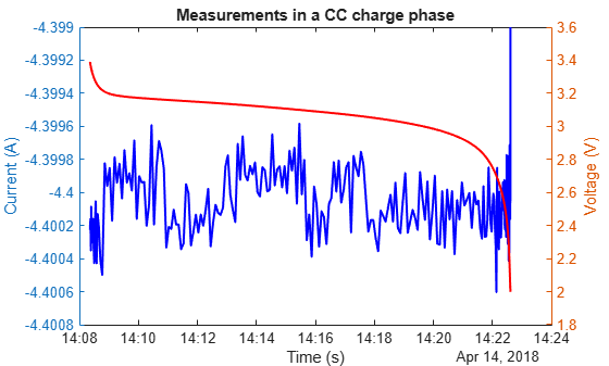
The current (in blue) stays relatively fixed about a center value. The voltage (in red) drops slowly throughout most of the charging, relative to the voltage axis on the right y axis, and sharply near the end of the CC phase.

Compute Differential Curves

Compute the differential curves for the battery data. The default value for NoiseTolerance is 1e-4. In this example, currents in the CC phase vary within 0.0016 A. Set NoiseTolerance to 0.002.

[dQdV, dVdQ, dTdV] = batteryDifferentialCurves(V,I,T,t,NoiseTolerance=0.002);

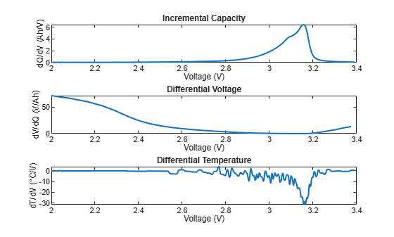
From the differential-curve data, plot the incremental capacity curve set.

figure
subplot(3,1,1)
plot(dQdV.interpolatedVoltage, dQdV.IC, 'LineWidth', 1.5)
xlabel('Voltage (V)')
ylabel('dQ/dV (Ah/V)')
title('Incremental Capacity')

subplot(3,1,2)
plot(dVdQ.interpolatedVoltage, dVdQ.DV, 'LineWidth', 1.5)
xlabel('Voltage (V)')
ylabel('dV/dQ (V/Ah)')
title('Differential Voltage')

subplot(3,1,3)
plot(dTdV.interpolatedVoltage, dTdV.DT, 'LineWidth', 1.5)
xlabel('Voltage (V)')
ylabel('dT/dV (°C/V)')
title('Differential Temperature')
set(findall(gcf,'Type','axes'), 'XLim', [2 3.4]);

Investigate Impact of Smoothing

By default, batteryDifferentialCurves computes the incremental capacity curves with Gaussian postsmoothing and no presmoothing. To visualize smoothing effects, compare differential temperature curves computed with:

1) No smoothing: Raw measurements

2) Presmoothing only: Smooths raw data before differentiation

3) Postsmoothing only: Smooths curves after differentiation

[~, ~, dTdV_raw] = batteryDifferentialCurves(V,I,T,t,"NoiseTolerance",0.002,... 
                  "PreSmoothingMethod", "none", "PostSmoothingMethod", "none");
[~, ~, dTdV_presmooth] = batteryDifferentialCurves(V,I,T,t,"NoiseTolerance",0.002,...
                  "PreSmoothingMethod", "gaussian", "PostSmoothingMethod", "none");
figure
plot(dTdV_raw.interpolatedVoltage, dTdV_raw.DT, ...
    'LineWidth', 1.5, 'DisplayName', 'Raw DT Curve');
hold on
grid on
plot(dTdV_presmooth.interpolatedVoltage, dTdV_presmooth.DT, ...
    'LineWidth', 1.5, 'DisplayName', 'Pre-Smoothed DT Curve');
plot(dTdV.interpolatedVoltage, dTdV.DT, ...
    'LineWidth', 1.5, 'DisplayName', 'Post-Smoothed DT Curve');
hold off

xlabel('Voltage (V)')
ylabel('dT/dV (°C/V)')
title('DT Curves (Raw vs Pre-Smoothed vs Post-Smoothed)')
xlim([2.6 3.3])
ylim([-60 40])

legend('Location','best')

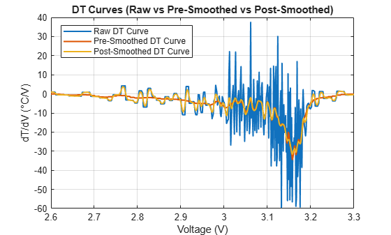
In the DT Curves plot, the unsmoothed curve exhibits noisy behavior. The curve with presmoothing is smoother, but excludes some detail. The curve with postsmoothing exhibits some of the noise of the unsmoothed curve, but retains more detail than the presmoothed curve.

The effectiveness of the smoothing techniques depend on the method and window size, which are controlled by the the name-value arguments: PreSmoothingMethod, PreSmoothingWindowSize, PostSmoothingMethod, and PostSmoothingWindowSize.

Investigate Impact of Interpolation Density in Curve Calculation

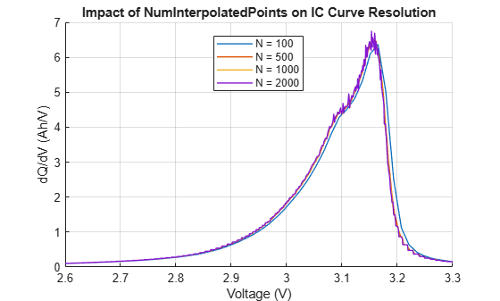
Visualize the impact of different interpolation point counts on incremental capacity curves without smoothing.

The number of interpolation points controls voltage resolution and curve smoothness. Increasing interpolation points can amplify noise in the derivative calculation, while too few points lead to under-sampling that distorts peak characteristics. This trade demonstrates why optimizing interpolation-point selection and smoothing parameters together is a good approach for accurate differential curve analysis.

interpolationPoints = [100, 500, 1000, 2000];

figure
hold on
grid on

for i = 1:numel(interpolationPoints)
    [dQdV, ~, ~] = batteryDifferentialCurves(V, I, T, t, ...
        NumInterpolatedPoints = interpolationPoints(i), ...
        PostSmoothingMethod  = 'none', ...
        NoiseTolerance       = 0.002);

    nPts = numel(dQdV.IC);

    plot(dQdV.interpolatedVoltage, dQdV.IC, ...
        'LineWidth', 1, ...
        'DisplayName', sprintf('N = %d', interpolationPoints(i)));
end

xlabel('Voltage (V)')
ylabel('dQ/dV (Ah/V)')
title('Impact of NumInterpolatedPoints on IC Curve Resolution')

xlim([2.6, 3.3])
legend('Location', 'best')
hold off