Estimate Lyapunov Exponent

R2026b

Interactively estimate the Lyapunov exponent of a uniformly sampled signal in the Live Editor

Description

The Estimate Lyapunov Exponent task lets you interactively estimate the Lyapunov exponent of a uniformly sampled signal. The task automatically generates MATLAB^® code for your live script. For more information about Live Editor tasks generally, see Add Interactive Tasks to Live Scripts.

Use the Lyapunov exponent to characterize the rate of separation of infinitesimally close trajectories in phase space to distinguish different attractors. The Lyapunov exponent is useful in quantifying the level of chaos in a system, which in turn can be used to detect potential faults. A negative Lyapunov exponent indicates convergence, while a positive Lyapunov exponents indicates divergence and chaos.

Open the Task

To add the Estimate Lyapunov Exponent task to a live script in the MATLAB Editor:

• On the Live Editor tab, select Task > Estimate Lyapunov Exponent.

• In a code block in your script, type a relevant keyword, such as Lyapunov or Lyapunov exponent. Select Estimate Lyapunov Exponent from the suggested command completions.

Examples

Estimate Lyapunov Exponent in the Live Editor

Use the Estimate Lyapunov Exponent task in the Live Editor to interactively estimate the Lyapunov exponent of a uniformly sampled signal. Experiment with different values for lag, embedding dimension, expansion range and mean period to align the linear fit line with the original data plot. The task automatically generates code reflecting your selections.

For this example, consider 'lyapExpData.mat' which contains reconstructed phase space signal phaseSpace sampled at 100 Hz.

load('lyapExpData.mat','phaseSpace')

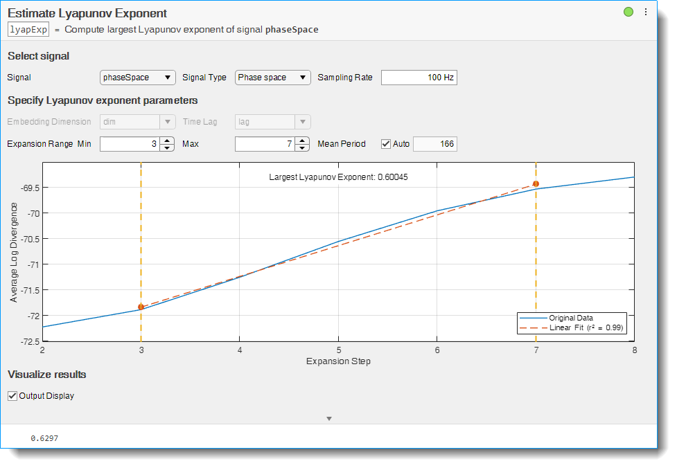
To estimate the Lyapunov exponent of the signal phaseSpace, open the Estimate Lyapunov Exponent task in the Live Editor. In the Live Editor tab, select Task > Estimate Lyapunov Exponent. In the task, select signal phaseSpace.

Since the selected signal is a phase space signal, select Phase space from the Signal Type menu. The signal was sampled at 100 Hz, so specify this value in the Sampling Rate field.

The Estimate Lyapunov Exponent task automatically computes the embedding dimension and lag from the phase space data and creates the Lyapunov exponent plot with default values for expansion range and mean period.

If your linear fit line does not align with the original data line using the default expansion range values, try different values in the Expansion Range Min, Expansion Range Max and Mean Period fields until the alignment is satisfactory. For this example, use the minimum value of 3 and maximum value of 7 for the best alignment. The default mean period value of 166 provides good alignment for the signal phaseSpace.

You can toggle displaying the output of the Lyapunov exponent value in the Live Editor output using the Output Display option.

The task generates code in your live script. The generated code reflects the parameters and options you specify. To see the generated code, click at the bottom of the task parameter area. The task expands to display the generated code.

By default, the generated code uses lyapExp as the name of the output variable. To specify a different output variable name, enter a new name in the summary line at the top of the task. For instance, change the name to lExponent.

The task updates the generated code to reflect the new variable name, and the new variable lExponent appears in the MATLAB® workspace. A negative Lyapunov exponent indicates convergence, while positive Lyapunov exponents demonstrate divergence and chaos. The magnitude of lExponent is an indicator of the rate of convergence or divergence of the infinitesimally close trajectories.

Related Examples

• Reconstruct Phase Space and Estimate Condition Indicators Using Live Editor Tasks

Parameters

Select Signal

Signal — Uniformly sampled time-domain signal

array | timetable

Select a uniformly sampled time-domain signal in array or timetable format. If the signal has multiple columns, the Estimate Lyapunov Exponent task computes the Lyapunov exponent by treating it as a multivariate signal. If the signal is a row vector, then the Estimate Lyapunov Exponent task treats it as a univariate signal.

Signal Type — Type of selected signal

'Time Domain' | 'Phase space'

Specify the type of the selected signal as either 'Time Domain' or 'Phase space'. If you specify the signal type as:

• 'Time Domain', then also specify the embedding dimension and time lag for your signal.

• 'Phase space', then the Estimate Correlation Dimension task automatically computes the embedding dimension and time lag using the phase space information.

Sampling Rate — Sampling frequency of the data set

2π (default) | scalar

Specify the sampling frequency of the data set as a scalar. The Estimate Lyapunov Exponent task uses a value of 2π or 6.283 Hz by default. When the signal data is in a timetable, the Estimate Lyapunov Exponent task infers the sampling rate from the data set.

Specify Lyapunov Exponent Parameters

Embedding Dimension — Number of dimensions of phase space vectors

scalar | vector

Specify the number of dimensions of phase space vectors as a scalar or vector from the MATLAB workspace. When you specify the embedding dimension as a scalar, then the Estimate Lyapunov Exponent task uses the same embedding dimension value to estimate the value of Lyapunov exponent for all the columns of the uniformly sampled signal.

The Embedding Dimension drop down is active only when you specify the signal type as 'Time Domain'. For phase space signals, the Estimate Lyapunov Exponent task automatically computes the embedding dimension from the phase space data.

If you do not know the value of embedding dimension for your signal, then you can compute it using the Reconstruct Phase Space task.

Time Lag — Time lag between successive phase vectors

scalar | vector

Specify time lag between successive phase vectors as a scalar or vector from the MATLAB workspace. When you specify the time lag as a scalar, then the Estimate Lyapunov Exponent task uses the same time delay value to estimate the value of Lyapunov exponent for all the columns of the uniformly sampled signal. If you specify the embedding dimension as a vector, then specify the time lag also as a vector of the same length.

The Time Lag drop down is active only when you specify the signal type as 'Time Domain'. For phase space signals, the Estimate Lyapunov Exponent task automatically computes the time lag from the phase space data.

If you do not know the value of time lag for your signal, then you can compute it using the Reconstruct Phase Space task.

Expansion Range Min — Minimum expansion step value

1 (default) | positive scalar integer

Specify the minimum expansion step value used to compute the expansion rate to estimate the Lyapunov exponent. Try different values such that the linear fit line aligns with the original data line in the plot.

Expansion Range Max — Maximum expansion step value

5 (default) | positive scalar integer

Specify the maximum expansion step value used to compute the expansion rate to estimate the Lyapunov exponent. Try different values such that the linear fit line aligns with the original data line in the plot.

Mean Period — Threshold value for nearest neighbor computation

ceil(fs/max(meanfreq(signal,sampling rate))) (default) | positive scalar integer

Specify the threshold value to compute the nearest neighbor i* for a point i to estimate the largest Lyapunov exponent. For more information, see lyapunovExponent.

Visualize Results

Output Display — Toggle result display in the Live Editor output

on (default) | off

Toggle to display the value of Lyapunov exponent in the Live Editor output.

Version History

Introduced in R2019b