Main Content

step

System object: phased.WidebandFreeSpace
Namespace: phased

Propagate wideband signal from point to point using free-space channel model

Syntax

prop_sig = step(sWBFS,sig,origin_pos,dest_pos,origin_vel,dest_vel)

Description

Note

Starting in R2016b, instead of using the step method to perform the operation defined by the System object™, you can call the object with arguments, as if it were a function. For example, y = step(obj,x) and y = obj(x) perform equivalent operations.

prop_sig = step(sWBFS,sig,origin_pos,dest_pos,origin_vel,dest_vel) returns the resulting signal, prop_sig, when a wideband signal sig propagates through a free-space channel from the origin_pos position to the dest_pos position. Either the origin_pos or dest_pos arguments can specify more than one point but you cannot specify both as having multiple points. The velocity of the signal origin is specified in origin_vel and the velocity of the signal destination is specified in dest_vel. The dimensions of origin_vel and dest_vel must agree with the dimensions of origin_pos and dest_pos, respectively.

Electromagnetic fields propagated through a free-space channel can be polarized or nonpolarized. For nonpolarized fields, such as acoustic fields, the propagating signal field, sig, is a vector or matrix. When the fields are polarized, sig is a struct array. Every structure element represents an electric field vector signal.

Note

The object performs an initialization the first time the object is executed. This initialization locks nontunable properties and input specifications, such as dimensions, complexity, and data type of the input data. If you change a nontunable property or an input specification, the System object issues an error. To change nontunable properties or inputs, you must first call the release method to unlock the object.

Input Arguments

expand all

Wideband free space propagator, specified as a System object.

Example: phased.WidebandFreeSpace

  • Wideband nonpolarized signal, specified as an M-by-N complex-valued matrix. Each column contains a signal propagated along one of the free-space paths.

  • Wideband polarized signal, specified as a 1-by-N struct array containing complex-valued fields. Each struct element contains an M-by-1 column vector of electromagnetic field components (sig.X,sig.Y,sig.Z) representing a polarized signal propagating along one of the free-space paths.

The quantity M is the number of signal samples and N is the number of free-space channels. Each channel corresponds to a source-destination pair.

The size of the first dimension of the input matrix can vary to simulate a changing signal length. A size change can occur, for example, in the case of a pulse waveform with variable pulse repetition frequency.

For polarized fields, each struct element contains three M-by-1 complex-valued column vectors, sig.X, sig.Y, and sig.Z. These vectors represent the x, y, and z Cartesian components of the polarized signal.

The size of the first dimension of the matrix fields within the struct can vary to simulate a changing signal length such as a pulse waveform with variable pulse repetition frequency.

Example: [1,1;j,1;0.5,0]

Data Types: double
Complex Number Support: Yes

Origin of the signal or signals, specified as a 3-by-1 real-valued column vector or 3-by-N real-valued matrix. Position units are in meters. The quantity N is the number of free-space channels. If origin_pos is a column vector, it takes the form [x;y;z]. If origin_pos is a matrix, each column specifies a different signal origin and has the form [x;y;z].

You cannot specify both origin_pos and dest_pos as matrices. At least one must be a 3-by-1 column vector.

Example: [1000;100;500]

Data Types: double

Destination of the signal or signals, specified as a 3-by-1 real-valued column vector or 3-by-N real-valued matrix. Position units are in meters. The quantity N is the number of free-space channels. If dest_pos is a 3-by-1 column vector, it takes the form [x;y;z]. If dest_pos is a matrix, each column specifies a different signal destination and takes the form [x;y;z].

You cannot specify both origin_pos and dest_pos as matrices. At least one must be a 3-by-1 column vector.

Example: [0;0;0]

Data Types: double

Velocity of signal origin, specified as a real-valued 3-by-1 column vector or real-valued 3-by-N matrix. Velocity units are in meters per second. The dimension of origin_vel must match the dimension of origin_pos. If origin_vel is a column vector, it takes the form [Vx;Vy;Vz]. If origin_vel is a 3–by-N matrix, each column specifies a different origin velocity and has the form [Vx;Vy;Vz].

Example: [10;0;5]

Data Types: double

Velocity of signal destinations, specified as a 3-by-1 column vector or 3–by-N matrix. Velocity units are in meters per second. The dimension of dest_vel must match the dimension of dest_pos. If dest_vel is a column vector, it takes the form [Vx;Vy;Vz]. If dest_vel is a 3–by-N matrix, each column specifies a different destination velocity and has the form [Vx;Vy;Vz].

Example: [0;0;0]

Data Types: double

Output Arguments

expand all

  • Wideband nonpolarized signal, specified as an M-by-N complex-valued matrix. Each column contains a signal propagated along one of the free-space paths.

  • Wideband polarized signal, specified as a 1-by-N struct array containing complex-valued fields. Each struct element contains an M-by-1 column vector of electromagnetic field components (sig.X,sig.Y,sig.Z) representing a polarized signal propagating along one of the free-space paths.

The output prop_sig contains signal samples arriving at the signal destination within the current steptime frame. Whenever it takes longer than the current time frame for the signal to propagate from the origin to the destination, the output may not contain all contribution from the input. The next call to step will return more of the propagated signal.

Examples

expand all

Propagate a wideband signal with three tones in an underwater acoustic with constant speed of propagation. You can model this environment as free space. The center frequency is 100 kHz and the frequencies of the three tones are 75 kHz, 100 kHz, and 125 kHz, respectively. Plot the spectrum of the original signal and the propagated signal to observe the Doppler effect. The sampling frequency is 100 kHz.

c = 1500;
fc = 100e3;
fs = 100e3;
relfreqs = [-25000,0,25000];

Set up a stationary radar and moving target and compute the expected Doppler.

rpos = [0;0;0];
rvel = [0;0;0];
tpos = [30/fs*c; 0;0];
tvel = [45;0;0];
dop = -tvel(1)./(c./(relfreqs + fc));

Create a signal and propagate the signal to the moving target.

t = (0:199)/fs;
x = sum(exp(1i*2*pi*t.'*relfreqs),2);
channel = phased.WidebandFreeSpace(...
    'PropagationSpeed',c,...
    'OperatingFrequency',fc,...
    'SampleRate',fs);
y = channel(x,rpos,tpos,rvel,tvel);

Plot the spectra of the original signal and the Doppler-shifted signal.

periodogram([x y],rectwin(size(x,1)),1024,fs,'centered')
ylim([-150 0])
legend('original','propagated');

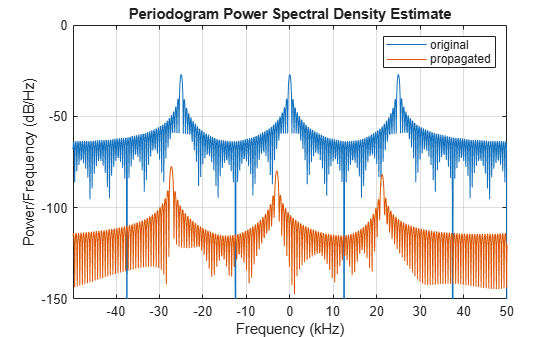
For this wideband signal, you can see that the magnitude of the Doppler shift increases with frequency. In contrast, for narrowband signals, the Doppler shift is assumed constant over the band.

References

[1] Proakis, J. Digital Communications. New York: McGraw-Hill, 2001.

[2] Skolnik, M. Introduction to Radar Systems. 3rd Ed. New York: McGraw-Hill

[3] Saakian, A. Radio Wave Propagation Fundamentals. Norwood, MA: Artech House, 2011.

[4] Balanis, C. Advanced Engineering Electromagnetics. New York: Wiley & Sons, 1989.

[5] Rappaport, T. Wireless Communications: Principles and Practice. 2nd Ed. New York: Prentice Hall, 2002.

Version History

Introduced in R2015b