pattern

System object: phased.ConformalArray
Namespace: phased

Plot conformal array pattern

Syntax

pattern(sArray,FREQ)
pattern(sArray,FREQ,AZ)
pattern(sArray,FREQ,AZ,EL)
pattern(___,Name,Value)
[PAT,AZ_ANG,EL_ANG] = pattern(___)


Description

pattern(sArray,FREQ) plots the 3-D array directivity pattern (in dBi) for the array specified in sArray. The operating frequency is specified in FREQ.

The integration used when computing array directivity has a minimum sampling grid of 0.1 degrees. If an array pattern has a beamwidth smaller than this, the directivity value will be inaccurate.

pattern(sArray,FREQ,AZ) plots the array directivity pattern at the specified azimuth angle.

pattern(sArray,FREQ,AZ,EL) plots the array directivity pattern at specified azimuth and elevation angles.

pattern(___,Name,Value) plots the array pattern with additional options specified by one or more Name,Value pair arguments.

[PAT,AZ_ANG,EL_ANG] = pattern(___) returns the array pattern in PAT. The AZ_ANG output contains the coordinate values corresponding to the rows of PAT. The EL_ANG output contains the coordinate values corresponding to the columns of PAT. If the 'CoordinateSystem' parameter is set to 'uv', then AZ_ANG contains the U coordinates of the pattern and EL_ANG contains the V coordinates of the pattern. Otherwise, they are in angular units in degrees. UV units are dimensionless.

Note

When you need to compute array or element directivity, you can either set the Type property to "directivity" in the pattern object function or use the directivity object function. For a small number of angular directions, it may be more computationally efficient to use the directivity object function. The pattern object function is more efficient for computing directivity for larger angular regions.

Input Arguments

sArray — Conformal array

System object™

Conformal array, specified as a phased.ConformalArray System object.

Example: sArray= phased.ConformalArray;

FREQ — Frequency for computing directivity and patterns

positive scalar | 1-by-L real-valued row vector

Frequencies for computing directivity and patterns, specified as a positive scalar or 1-by-L real-valued row vector. Frequency units are in hertz.

• For an antenna, microphone, or sonar hydrophone or projector element, FREQ must lie within the range of values specified by the FrequencyRange or FrequencyVector property of the element. Otherwise, the element produces no response and the directivity is returned as –Inf. Most elements use the FrequencyRange property except for phased.CustomAntennaElement and phased.CustomMicrophoneElement, which use the FrequencyVector property.

• For an array of elements, FREQ must lie within the frequency range of the elements that make up the array. Otherwise, the array produces no response and the directivity is returned as –Inf.

Example: [1e8 2e6]

Data Types: double

AZ — Azimuth angles

[-180:180] (default) | 1-by-N real-valued row vector

Azimuth angles for computing directivity and pattern, specified as a 1-by-N real-valued row vector where N is the number of azimuth angles. Angle units are in degrees. Azimuth angles must lie between –180° and 180°.

The azimuth angle is the angle between the x-axis and the projection of the direction vector onto the xy plane. When measured from the x-axis toward the y-axis, this angle is positive.

Example: [-45:2:45]

Data Types: double

EL — Elevation angles

[-90:90] (default) | 1-by-M real-valued row vector

Elevation angles for computing directivity and pattern, specified as a 1-by-M real-valued row vector where M is the number of desired elevation directions. Angle units are in degrees. The elevation angle must lie between –90° and 90°.

The elevation angle is the angle between the direction vector and xy-plane. The elevation angle is positive when measured towards the z-axis.

Example: [-75:1:70]

Data Types: double

Name-Value Arguments

Specify optional pairs of arguments as Name1=Value1,...,NameN=ValueN, where Name is the argument name and Value is the corresponding value. Name-value arguments must appear after other arguments, but the order of the pairs does not matter.

Before R2021a, use commas to separate each name and value, and enclose Name in quotes.

CoordinateSystem — Plotting coordinate system

"polar" (default) | "rectangular" | "uv"

Plotting coordinate system of the pattern, specified as the comma-separated pair consisting of CoordinateSystem and one of "polar", "rectangular", or "uv". When CoordinateSystem is set to "polar" or "rectangular", the AZ and EL arguments specify the pattern azimuth and elevation, respectively. AZ values must lie between –180° and 180°. EL values must lie between –90° and 90°. If CoordinateSystem is set to "uv", AZ and EL then specify U and V coordinates, respectively. AZ and EL must lie between -1 and 1.

Example: "uv"

Data Types: char

Type — Displayed pattern type

"directivity" (default) | "efield" | "power" | "powerdb"

Displayed pattern type, specified as the equal-sign-separated pair consisting of Type and one of

• "directivity" — directivity pattern measured in dBi.

• "efield" — field pattern of the sensor or array. For acoustic sensors, the displayed pattern is for the scalar sound field.

• "power" — power pattern of the sensor or array defined as the square of the field pattern.

• "powerdb" — power pattern converted to dB.

Example: "powerdb"

Data Types: char

Orientation — Array orientation

[0;0;0]. (default) | 3-by-1 real-valued column vector

Array orientation, specified as a 3-by-1 real-valued column vector containing three rotation angles. The three angles define orthogonal rotations with respect to the x-, y-, and z-axes of the local coordinate system. To create the full orientation matrix, the orthogonal rotations are applied in this order:

1. a rotation around the positive x-axis by the angle θ_x.

2. a rotation around the positive y-axis by the angle θ_y.

3. a rotation around the positive z-axis by the angle θ_z.

Positive angles are defined using the right-handed rule. A positive angle defines a rotation that appears clockwise when looking towards the positive direction of the axis, and negative values when the rotation appears counter-clockwise. The right-hand rule is invoked by pointing the right-hand thumb along an axis. Then the other fingers of the right hand curl in the positive direction,

Normalize — Display normalize pattern

true (default) | false

Display normalized pattern, specified as the comma-separated pair consisting of Normalize and a Boolean. Set this parameter to true to display a normalized pattern. This parameter does not apply when you set Type to "directivity". Directivity patterns are already normalized.

Data Types: logical

ShowArray — View array geometry

false (default) | true

View the array geometry along with the 3D radiation pattern, specified as false or true.

Data Types: logical

ShowLocalCoordinates — Show local coordinate axes

true (default) | false

Show the local coordinate axes, specified as true or false.

Data Types: logical

ShowColorbar — Show colorbar

true (default) | false

Show the colorbar, specified as true or false.

Data Types: logical

Parent — Handle to axis

scalar

Handle to the axes along which the array geometry is displayed specified as a scalar.

PlotStyle — Plotting style

"overlay" (default) | "waterfall"

Plotting style, specified as the equal-sign-separated pair consisting of Plotstyle and either "overlay" or "waterfall". This parameter applies when you specify multiple frequencies in FREQ in 2-D plots. You can draw 2-D plots by setting one of the arguments AZ or EL to a scalar.

Data Types: char

Polarization — Polarized field component

'combined' (default) | 'H' | 'V'

Polarized field component to display, specified as the comma-separated pair consisting of 'Polarization' and 'combined', 'H', or 'V'. This parameter applies only when the sensors are polarization-capable and when the 'Type' parameter is not set to 'directivity'. This table shows the meaning of the display options.

'Polarization'	Display
'combined'	Combined H and V polarization components
'H'	H polarization component
'V'	V polarization component

Example: 'V'

Data Types: char

PropagationSpeed — Signal propagation speed

speed of light (default) | positive scalar

Signal propagation speed, specified as the comma-separated pair consisting of PropagationSpeed and a positive scalar in meters per second.

Example: PropagationSpeed="physconst('LightSpeed')"

Data Types: double

Weights — Array weights

1 (default) | N-by-1 complex-valued column vector | N-by-L complex-valued matrix

Array weights, specified as the comma-separated pair consisting of 'Weights' and an N-by-1 complex-valued column vector or N-by-L complex-valued matrix. Array weights are applied to the elements of the array to produce array steering, tapering, or both. The dimension N is the number of elements in the array. The dimension L is the number of frequencies specified by FREQ.

Weights Dimension	FREQ Dimension	Purpose
N-by-1 complex-valued column vector	Scalar or 1-by-L row vector	Applies a set of weights for the single frequency or for all L frequencies.
N-by-L complex-valued matrix	1-by-L row vector	Applies each of the L columns of 'Weights' for the corresponding frequency in FREQ.

Note

Use complex weights to steer the array response toward different directions. You can create weights using the phased.SteeringVector System object or you can compute your own weights. In general, you apply Hermitian conjugation before using weights in any Phased Array System Toolbox™ function or System object such as phased.Radiator or phased.Collector. However, for the directivity, pattern, patternAzimuth, and patternElevation methods of any array System object use the steering vector without conjugation.

Example: 'Weights',ones(N,M)

Data Types: double
Complex Number Support: Yes

Output Arguments

PAT — Array pattern

M-by-N real-valued matrix

Array pattern, returned as an M-by-N real-valued matrix. The dimensions of PAT correspond to the dimensions of the output arguments AZ_ANG and EL_ANG.

AZ_ANG — Azimuth angles

scalar | 1-by-N real-valued row vector

Azimuth angles for displaying directivity or response pattern, returned as a scalar or 1-by-N real-valued row vector corresponding to the dimension set in AZ. The columns of PAT correspond to the values in AZ_ANG. Units are in degrees.

EL_ANG — Elevation angles

scalar | 1-by-M real-valued row vector

Elevation angles for displaying directivity or response, returned as a scalar or 1-by-M real-valued row vector corresponding to the dimension set in EL. The rows of PAT correspond to the values in EL_ANG. Units are in degrees.

Examples

Plot Power Pattern of 8-Element Uniform Circular Array

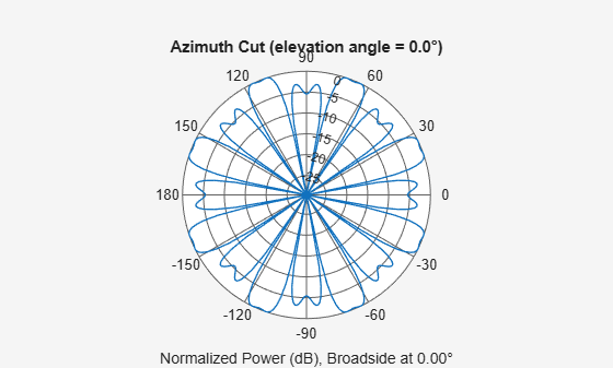
Using the ConformalArray System object™, construct an 8-element uniform circular array (UCA) of isotropic antenna elements. Plot a normalized azimuth power pattern at 0 degrees elevation. Assume the operating frequency is 1 GHz and the wave propagation speed is the speed of light.

N = 8;
azang = (0:N-1)*360/N-180;
sCA = phased.ConformalArray(...
    'ElementPosition',[cosd(azang);sind(azang);zeros(1,N)],...
    'ElementNormal',[azang;zeros(1,N)]);
fc = 1e9;
c = physconst('LightSpeed');
pattern(sCA,fc,[-180:180],0,...
    'PropagationSpeed',c,'Type','powerdb',...
    'CoordinateSystem','polar')

Plot Pattern of 31-Element Uniform Circular Sonar Array

Construct a 31-element acoustic uniform circular sonar array (UCA) using the ConformalArray System object™. Assume the array is one meter in diameter. Using the ElevationAngles parameter, restrict the display to +/-40 degrees in 0.1 degree increments. Assume the operating frequency is 4 kHz. A typical value for the speed of sound in seawater is 1500.0 m/s.

Construct the array

N = 31;
theta = (0:N-1)*360/N-180;
Radius = 0.5;
sMic = phased.OmnidirectionalMicrophoneElement(...
    'FrequencyRange',[0,10000],'BackBaffled',true);
sArray = phased.ConformalArray('Element',sMic,...
    'ElementPosition',Radius*[zeros(1,N);cosd(theta);sind(theta)],...
    'ElementNormal',[ones(1,N);zeros(1,N)]);

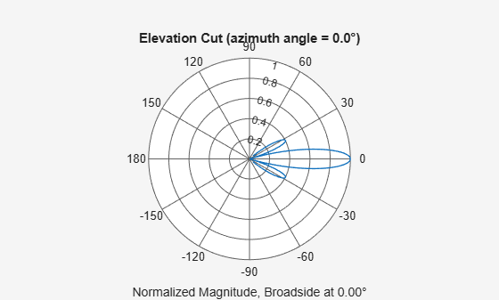
Plot the magnitude pattern

fc = 4000;
c = 1500.0;
pattern(sArray,fc,0,[-40:0.1:40],...
    'PropagationSpeed',c,...
    'CoordinateSystem','polar',...
    'Type','efield')

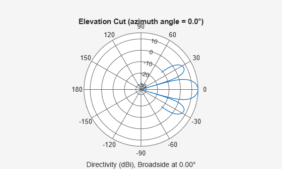
Plot the directivity pattern

pattern(sArray,fc,0,[-40:0.1:40],...
    'PropagationSpeed',c,...
    'CoordinateSystem','polar',...
    'Type','directivity')

More About

Directivity

Directivity describes the directionality of the radiation pattern of a sensor element or array of sensor elements.

Higher directivity is desired when you want to transmit more radiation in a specific direction. Directivity is the ratio of the transmitted radiant intensity in a specified direction to the radiant intensity transmitted by an isotropic radiator with the same total transmitted power

$$D=4\pi \frac{U_{\text{rad}}\left(\theta ,\phi \right)}{P_{\text{total}}}$$

where U_rad(θ,φ) is the radiant intensity of a transmitter in the direction (θ,φ) and P_total is the total power transmitted by an isotropic radiator. For a receiving element or array, directivity measures the sensitivity toward radiation arriving from a specific direction. The principle of reciprocity shows that the directivity of an element or array used for reception equals the directivity of the same element or array used for transmission. When converted to decibels, the directivity is denoted as dBi. For information on directivity, read the notes on Element Directivity and Array Directivity.

Convert plotResponse to pattern

For antenna, microphone, and array System objects, the pattern method replaces the plotResponse method. In addition, two new simplified methods exist just to draw 2-D azimuth and elevation pattern plots. These methods are patternAzimuth and patternElevation.

The following table is a guide for converting your code from using plotResponse to pattern. Notice that some of the inputs have changed from input arguments to Name-Value pairs and conversely. The general pattern method syntax is

pattern(H,FREQ,AZ,EL,'Name1','Value1',...,'NameN','ValueN')

plotResponse Inputs	plotResponse Description	pattern Inputs
H argument	Antenna, microphone, or array System object.	H argument (no change)
FREQ argument	Operating frequency.	FREQ argument (no change)
V argument	Propagation speed. This argument is used only for arrays.	'PropagationSpeed' name-value pair. This parameter is only used for arrays.
'Format' and 'RespCut' name-value pairs	These options work together to let you create a plot in angle space (line or polar style) or UV space. They also determine whether the plot is 2-D or 3-D. This table shows you how to create different types of plots using plotResponse. Display space   Angle space (2D) Set 'RespCut' to 'Az' or 'El'. Set 'Format' to 'line' or 'polar'. Set the display axis using either the 'AzimuthAngles' or 'ElevationAngles' name-value pairs. Angle space (3D) Set 'RespCut' to '3D'. Set 'Format' to 'line' or 'polar'. Set the display axis using both the 'AzimuthAngles' and'ElevationAngles' name-value pairs. UV space (2D) Set 'RespCut' to'U'. Set 'Format' to 'UV'. Set the display range using the 'UGrid' name-value pair. UV space (3D) Set 'RespCut' to'3D'. Set 'Format' to 'UV'. Set the display range using both the 'UGrid' and 'VGrid' name-value pairs.	'CoordinateSystem' name-value pair used together with the AZ and EL input arguments. 'CoordinateSystem' has the same options as the plotResponse method 'Format'name-value pair, except that 'line' is now named 'rectangular'. The table shows how to create different types of plots using pattern. Display space   Angle space (2D) Set 'Coordinate System' to 'rectangular' or 'polar'. Specify either AZ or EL as a scalar. Angle space (3D) Set 'Coordinate System' to 'rectangular' or 'polar'. Specify both AZ and EL as vectors. UV space (2D) Set 'Coordinate System' to 'uv'. Use AZ to specify a U-space vector. Use EL to specify a V-space scalar. UV space (3D) Set 'Coordinate System' to 'uv'. Use AZ to specify a U-space vector. Use EL to specify a V-space vector. If you set CoordinateSystem to 'uv', enter the UV grid values using AZ and EL.
'CutAngle' name-value pair	Constant angle at to take an azimuth or elevation cut. When producing a 2-D plot and when 'RespCut' is set to 'Az' or 'El', use 'CutAngle' to set the slice across which to view the plot.	No equivalent name-value pair. To create a cut, specify either AZ or EL as a scalar, not a vector.
'NormalizeResponse' name-value pair	Normalizes the plot. When 'Unit' is set to 'dbi', you cannot specify 'NormalizeResponse'.	Use the 'Normalize' name-value pair. When 'Type' is set to 'directivity' you cannot specify 'Normalize'.
'OverlayFreq' name-value pair	Plot multiple frequencies on the same 2-D plot. Available only when 'Format' is set to 'line' or 'uv' and 'RespCut' is not set to '3D'. The value true produces an overlay plot and the value false produces a waterfall plot.	'PlotStyle' name-value pair plots multiple frequencies on the same 2-D plot. The values 'overlay' and 'waterfall' correspond to 'OverlayFreq' values of true and false. The option 'waterfall' is allowed only when 'CoordinateSystem' is set to 'rectangular' or 'uv'.
'Polarization' name-value pair	Determines how to plot polarized fields. Options are 'None', 'Combined', 'H', or 'V'.	'Polarization' name-value pair determines how to plot polarized fields. The 'None' option is removed. The options 'Combined', 'H', or 'V' are unchanged.
'Unit' name-value pair	Determines the plot units. Choose 'db', 'mag', 'pow', or 'dbi', where the default is 'db'.	'Type' name-value pair, uses equivalent options with different names plotResponse pattern 'db' 'powerdb' 'mag' 'efield' 'pow' 'power' 'dbi' 'directivity'
'Weights' name-value pair	Array element tapers (or weights).	'Weights' name-value pair (no change).
'AzimuthAngles' name-value pair	Azimuth angles used to display the antenna or array response.	AZ argument
'ElevationAngles' name-value pair	Elevation angles used to display the antenna or array response.	EL argument
'UGrid' name-value pair	Contains U coordinates in UV-space.	AZ argument when 'CoordinateSystem' name-value pair is set to 'uv'
'VGrid' name-value pair	Contains V-coordinates in UV-space.	EL argument when 'CoordinateSystem' name-value pair is set to 'uv'

Array axes and normals

The U/V coordinate system is determined by the array type and the array orientation. The Phased Array System Toolbox offers four basic array shapes: ULA, URA, UCA, and Conformal.

• For the phased.ULA System object use the ArrayAxis property to select the array orientation as "x", "y", or "z". The ArrayAxis property determines the elements layout, the normal direction of the array, and the orientation of the U/V space as shown in the table here:

  ULA Array

  ArrayAxis property value	Array element positions	Array normal	U/V space for ULA	U/V positive hemisphere for ULA	Plot of U/V space for ULA in 3D space
  "x"	x-axis	positive y-axis	xz-plane	y≥0
  "y"	y-axis	positive x-axis	yz-plane	x≥0
  "z"	z-axis	positive x-axis	yz-plane	x≥0

• For the phased.URA or phased.UCA System objects use the ArrayNormal property to select the array orientation as "x", "y", or "z". The ArrayNormal property determines the elements layout, the normal direction of the array, and the orientation of the U/V space as shown in the table here:

  URA and UCA Arrays

  ArrayNormal property value	Array element positions	Array normal	U/V space for URA/UCA	U/V positive hemisphere for URA/UCA	Plot of U/V space for URA/UCA in 3D space
  "z"	xy-plane	positive z-axis	xy-plane	z≥0
  "y"	xz-plane	positive y-axis	xz-plane	y≥0
  "x"	yz-plane	positive x-axis	yz-plane	x≥0

• For the phased.ConformalArray System object, uses the ElementPosition property to determine the elements layout, the normal direction of the array, and the orientation of the U/V space as shown in the table here:

  Conformal Array

  Array element positions	Array normal	U/V space for conformal array	U/V positive hemisphere for conformal array	Plot of U/V space for conformal array in 3D space
  Arbitrary in 3D space ElementPosition	positive x-axis	yz-plane	x≥0

Version History

Introduced in R2015a

R2024b: Array axis definitions

Enhanced definitions of array axes and normals.