Tapering, Thinning and Arrays with Different Sensor Patterns
This example shows how to apply tapering and model thinning on different array configurations. It also demonstrates how to create arrays with different element patterns.
ULA Tapering
This section shows how to apply a Taylor window on the elements of a uniform linear array (ULA) in order to reduce the sidelobe levels.
%set the random seed
rs = rng(6);

% Create a ULA antenna of 20 elements.
N = 20;
ula = phased.ULA(N);

% Clone the ideal ULA
taperedULA = clone(ula);

% Calculate and assign the taper
nbar = 5; sll = -20;
taperedULA.Taper = taylorwin(N,nbar,sll).';
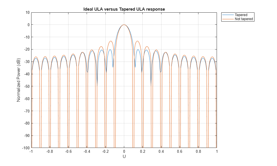
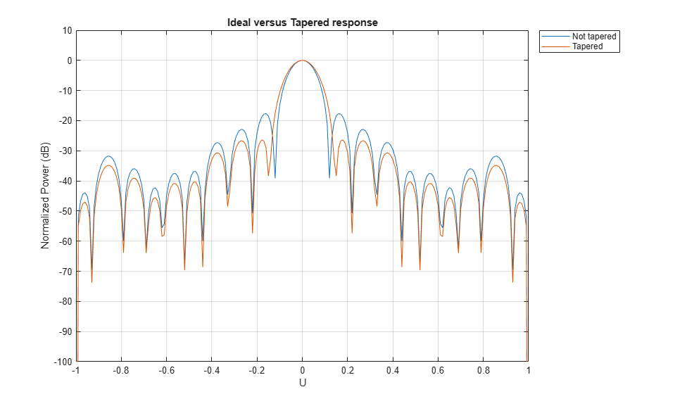
Compare the response of the tapered to the untapered array. Notice how the sidelobes of the tapered ULA are lower.
helperCompareResponses(taperedULA,ula, ...
                       'Ideal ULA versus Tapered ULA response', ...
                       {'Tapered','Not tapered'});
ULA Thinning
This section shows how to model thinning using tapering. When thinning, each element of the array has a certain probability of being deactivated or removed. The taper values can be either 0, for an inactive element, or 1 for an active element. Here, the probability of keeping the element is proportional to the value of the Taylor window at that element.
% Get that previously computed taper values corresponding to a Taylor
% window
taper = taperedULA.Taper;

% Create a random vector uniformly distributed between 0 and 1
randvect =  rand(size(taper));

% Compute the taper values whose probability of being 1 is equal to
% the value of the normalized Taylor window at the corresponding sensor.
thinningTaper = zeros(size(taper));
thinningTaper(randvect<taper/max(taper)) = 1;

% Apply thinning
thinnedULA = clone(ula);
thinnedULA.Taper = thinningTaper;
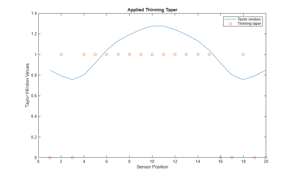
The following plot shows how the thinning taper values are distributed. Notice on the edges when the window level goes down, the number of inactive sensors is up.
plot(taper)
hold on
plot(thinningTaper,'o')
hold off
legend('Taylor window','Thinning taper')
title('Applied Thinning Taper');xlabel('Sensor Position');
ylabel('Taylor Window Values');
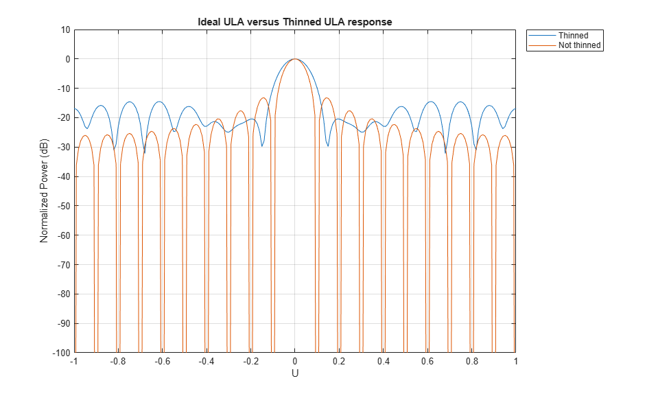
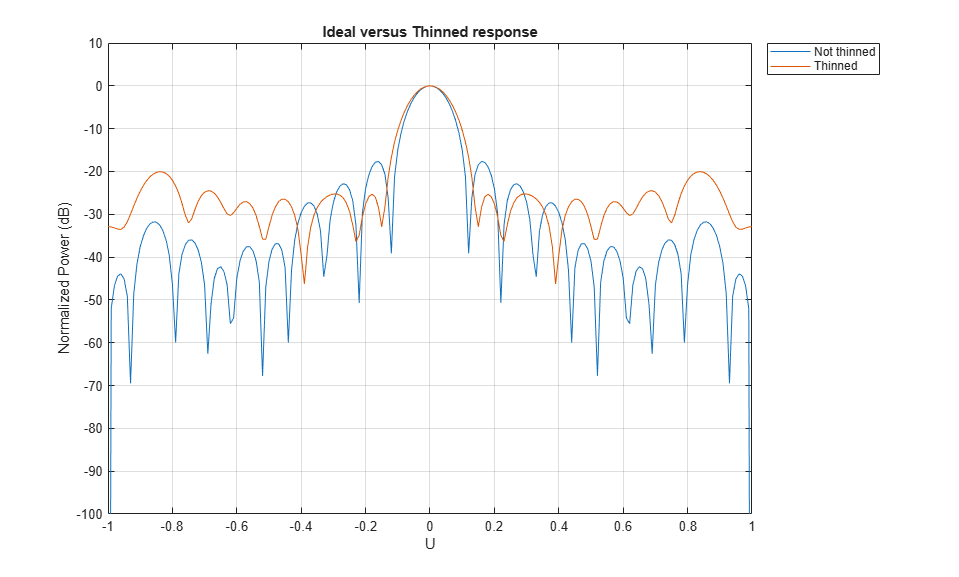
Compare the response of the thinned to the ideal array. Notice how the sidelobes of the thinned ULA are lower.
helperCompareResponses(thinnedULA,ula, ...
                       'Ideal ULA versus Thinned ULA response', ...
                       {'Thinned','Not thinned'});
URA Tapering
This section shows how to apply a Taylor window along both dimensions of a 13 by 10 uniform rectangular array (URA).
uraSize = [13,10];
heterogeneousURA = phased.URA(uraSize);

nbar=2; sll = -20;

% along the z axis
twinz = taylorwin(uraSize(1),nbar,sll);

% along the y axis
twiny = taylorwin(uraSize(2),nbar,sll);

% Get the total taper values by multiplying the vectors of both dimensions
tap = twinz*twiny.';

% Apply the taper
taperedURA = clone(heterogeneousURA);
taperedURA.Taper = tap;
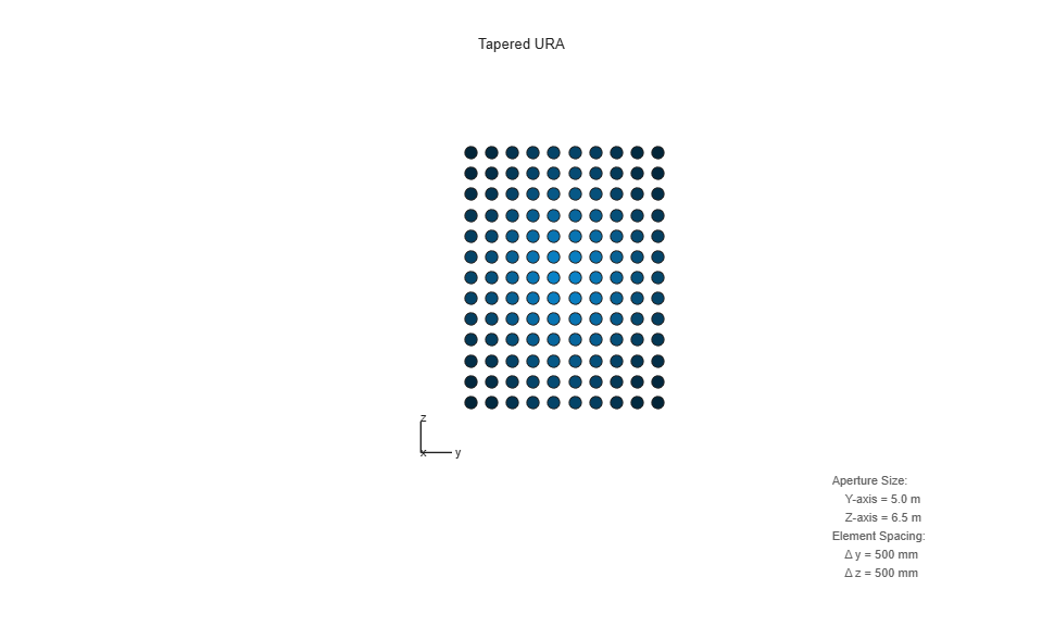
View the sensor's color brightness in proportion to the taper magnitudes.
viewArray(taperedURA,'Title','Tapered URA','ShowTaper',true);
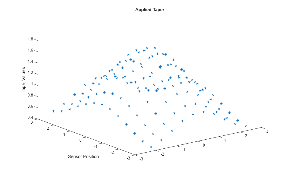
Plot the taper values at each sensor in 3d space.
clf
pos = getElementPosition(taperedURA);
plot3(pos(2,:),pos(3,:),taperedURA.Taper(:),'*');
title('Applied Taper');ylabel('Sensor Position');zlabel('Taper Values');
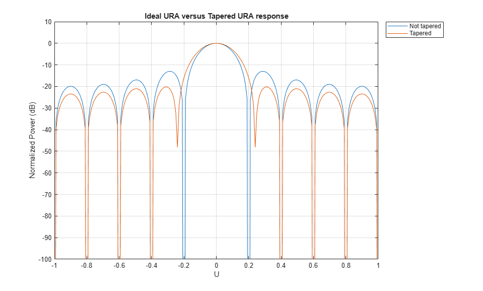
Compare the response of the tapered to the untapered array. Notice how the sidelobes of the tapered URA are lower.
helperCompareResponses(heterogeneousURA,taperedURA, ...
                       'Ideal URA versus Tapered URA response', ...
                       {'Not tapered','Tapered'});

Circular Planar Tapering
This section shows how to apply a taper on a circular planar array with a radius of 5 meters and distance between elements of 0.5 meters.
radius = 5; dist = 0.5;
numElPerSide = radius*2/dist;

% Get the positions of the smallest URA which could fit the circular planar
% array
pos = getElementPosition(phased.URA(numElPerSide,dist));

% Remove all elements in URA which are outside the circle
elemToRemove = sum(pos.^2) > radius^2;
pos(:,elemToRemove) = [];

% Create the circular planar array
circularPlanarArray = phased.ConformalArray('ElementPosition',pos,...
                           'ElementNormal',[0;0]*ones(1,size(pos,2)));
Apply a circular Taylor window.
taperedCircularPlanarArray = clone(circularPlanarArray);
nbar=3; sll = -25;

taperedCircularPlanarArray.Taper = taylortaperc(pos,2*radius,nbar,sll).';
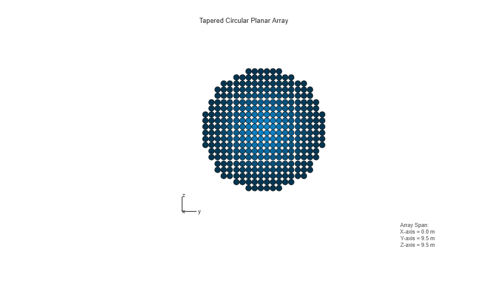
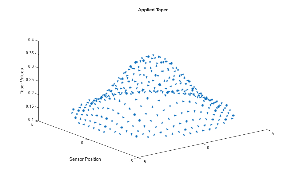
View the array and plot the taper values at each sensor.
viewArray(taperedCircularPlanarArray,...
    'Title','Tapered Circular Planar Array','ShowTaper',true)
clf
plot3(pos(2,:),pos(3,:),taperedCircularPlanarArray.Taper,'*');
title('Applied Taper');ylabel('Sensor Position');zlabel('Taper Values');
Compare the response of the tapered to the untapered array. Notice how the sidelobes of the tapered array are lower.
helperCompareResponses(circularPlanarArray,taperedCircularPlanarArray, ...
                       'Ideal versus Tapered response', ...
                       {'Not tapered','Tapered'});
Circular Planar Thinning
Calculate the thinning taper values similar to the ULA section.
taper = taperedCircularPlanarArray.Taper;
randvect = rand(size(taper));
thinningTaper = zeros(size(taper));
thinningTaper(randvect<taper/max(max(taper))) = 1;

thinnedCircularPlanarArray = clone(circularPlanarArray);
thinnedCircularPlanarArray.Taper = thinningTaper;
View the array and compare the response of the thinned to the ideal array.
viewArray(thinnedCircularPlanarArray,'ShowTaper',true)
clf;
helperCompareResponses(circularPlanarArray,thinnedCircularPlanarArray, ...
                       'Ideal versus Thinned response', ...
                       {'Not thinned','Thinned'});

Multiple Element Patterns in URA
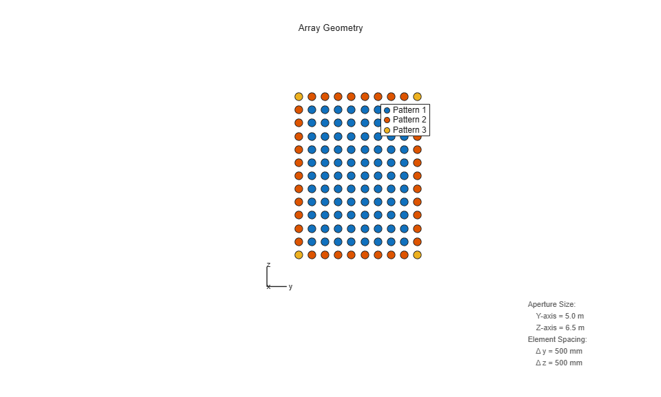
This section shows how to create a 13 by 10 URA with sensor patterns on the edges and corners different than the patterns of the remaining sensors. This ability could be used to model coupling effects.
Create three different cosine patterns with the following azimuth and elevation cosine exponents [azim exponent, elev exponent]: [2, 2] for the edges, [4, 4] for the corners, and [1.5, 1.5] for the main sensors.
mainAntenna = phased.CosineAntennaElement('CosinePower',[1.5 1.5]);
edgeAntenna = phased.CosineAntennaElement('CosinePower',[2 2]);
cornerAntenna = phased.CosineAntennaElement('CosinePower',[4 4]);
Map the sensors to the patterns.
uraSize = [13,10];

% Create a cell array which includes all the patterns
patterns = {mainAntenna, edgeAntenna, cornerAntenna};

% Initialize all sensors to first pattern.
patternMap = ones(uraSize);

% Set the edges to the second pattern.
patternMap([1 end],2:end-1) = 2;
patternMap(2:end-1,[1 end]) = 2;

% Set the corners to the third pattern.
patternMap([1 end],[1 end]) = 3;

% Create the URA

heterogeneousURA = phased.HeterogeneousURA('ElementSet' , patterns, ...
                               'ElementIndices', patternMap);
View the pattern layout in the array.
helperViewPatternArray(heterogeneousURA);
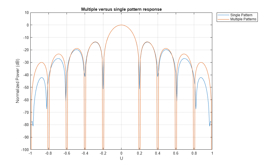
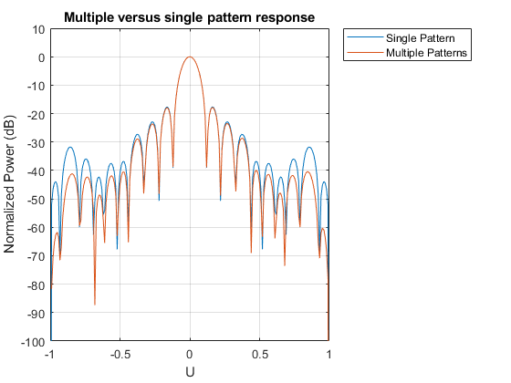
Compare the response of the multiple pattern array to the single pattern array.
clf;
helperCompareResponses( heterogeneousURA, ...
                        phased.URA(uraSize,'Element',mainAntenna), ...
                        'Multiple versus single pattern response', ...
                        {'Single Pattern','Multiple Patterns'});
Multiple Element Patterns in Circular Planar Arrays
This section shows how to set the pattern of sensors located more than 4 meters from the center of the array.
% Create a cell array which includes all the patterns
patterns = {mainAntenna, edgeAntenna};

% Get positions
pos = getElementPosition(circularPlanarArray);

% Initialize all sensors to first pattern in sensorPatterns.
patternMap = ones(1,size(pos,2));

% Get the indexed of the sensors more than 4 meters away from the center.
sensorIdx = find(sum(pos.^2) > 4^2);

% Set the edges to the second pattern in sensorPatterns.
patternMap(sensorIdx) = 2;

% Set the corresponding properties
heterogeneousCircularPlanarArray = ...
    phased.HeterogeneousConformalArray('ElementPosition',pos,...
                            'ElementNormal',[1;0]*ones(1,size(pos,2)),...
                            'ElementSet' , patterns, ...
                            'ElementIndices', patternMap);
View the pattern layout in the array.
helperViewPatternArray(heterogeneousCircularPlanarArray);
Compare the response of the multiple pattern array to the single pattern array.
clf;
helperCompareResponses(circularPlanarArray,...
    heterogeneousCircularPlanarArray,...
    'Multiple versus single pattern response',...
    {'Single Pattern','Multiple Patterns'});

% reset the random seed
rng(rs)
Summary
This example demonstrated how to apply taper values and model thinning using taper values for different array configurations. It also showed how to create arrays with different element patterns.
You can also select a web site from the following list:
Americas
- América Latina (Español)
- Canada (English)
- United States (English)
Europe
- Belgium (English)
- Denmark (English)
- Deutschland (Deutsch)
- España (Español)
- Finland (English)
- France (Français)
- Ireland (English)
- Italia (Italiano)
- Luxembourg (English)
- Netherlands (English)
- Norway (English)
- Österreich (Deutsch)
- Portugal (English)
- Sweden (English)
- Switzerland
- United Kingdom (English)