Simultaneous Range and Speed Estimation Using MFSK Waveform
This example compares triangle sweep frequency-modulated continuous (FMCW) and multiple frequency-shift keying (MFSK) waveforms used for simultaneous range and speed estimation for multiple targets. The MFSK waveform is specifically designed for automotive radar systems used in advanced driver assistance systems (ADAS). It is particularly appealing in multitarget scenarios because it does not introduce ghost targets.
Triangle Sweep FMCW Waveform
In the Automotive Adaptive Cruise Control Using FMCW Technology (Radar Toolbox) example an automotive radar system is designed to perform range estimation for an automatic cruise control system. In the latter part of that example, a triangle sweep FMCW waveform is used to estimate the range and speed of the target vehicle simultaneously.
Although the triangle sweep FMCW waveform elegantly solves the range-Doppler coupling issue for a single target, its processing becomes complicated in multitarget situations. The next section shows how a triangle sweep FMCW waveform behaves when two targets are present.
The scene includes a car 50 m away from the radar, traveling at 96 km/h along the same direction as the radar, and a truck at 55 m away, traveling at 70 km/h in the opposite direction. The radar itself is traveling at 60 km/h.
rng(2015);
[fmcwwaveform,target,tgtmotion,channel,transmitter,receiver, ...
    sensormotion,c,fc,lambda,fs,maxbeatfreq] = helperMFSKSystemSetup;
Next, simulate the radar echo from the two vehicles. The FMCW waveform has a sweep bandwidth of 150 MHz so the range resolution is 1 meter. Each up or down sweep takes 1 millisecond, so each triangle sweep takes 2 milliseconds. Note that only one triangle sweep is needed to perform the joint range and speed estimation.
Nsweep = 2;
xr = helperFMCWSimulate(Nsweep,fmcwwaveform,sensormotion,tgtmotion, ...
    transmitter,channel,target,receiver);
Although the system needs a 150 MHz bandwidth, the maximum beat frequency is much less. This means that at the processing side, one can decimate the signal to a lower frequency to ease the hardware requirements. The beat frequencies are then estimated using the decimated signal.
dfactor = ceil(fs/maxbeatfreq)/2;
fs_d = fs/dfactor;
fbu_rng = rootmusic(decimate(xr(:,1),dfactor),2,fs_d);
fbd_rng = rootmusic(decimate(xr(:,2),dfactor),2,fs_d);
Now there are two beat frequencies from the up sweep and two beat frequencies from the down sweeps. Since any pair of beat frequencies from an up sweep and a down sweep can define a target, there are four possible combinations of range and Doppler estimates, yet only two of them are associated with the real targets.
sweep_slope = fmcwwaveform.SweepBandwidth/fmcwwaveform.SweepTime;
rng_est = beat2range([fbu_rng fbd_rng;fbu_rng flipud(fbd_rng)], ...
    sweep_slope,c)
rng_est = 4×1
49.9802
54.9406
64.2998
40.6210
The remaining two are what is often referred to as ghost targets. The relationship between real targets and ghost targets can be better explained using time-frequency representation.

As shown in the figure, each intersection of an up sweep return and a down sweep return indicates a possible target. So it is critical to distinguish between the true targets and the ghost targets. To solve this ambiguity, one can transmit additional FMCW signals with different sweep slopes. Since only the true targets will occupy the same intersection in the time-frequency domain, the ambiguity is resolved. However, this approach significantly increases the processing complexity as well as the processing time needed to obtain the valid estimates.
MFSK Waveform
Multiple frequency shift keying (MFSK) waveform [1] is designed for the automotive radar to achieve simultaneous range and Doppler estimation under the multiple targets situation without falling into the trap of ghost targets. Its time-frequency representation is shown in the following figure.
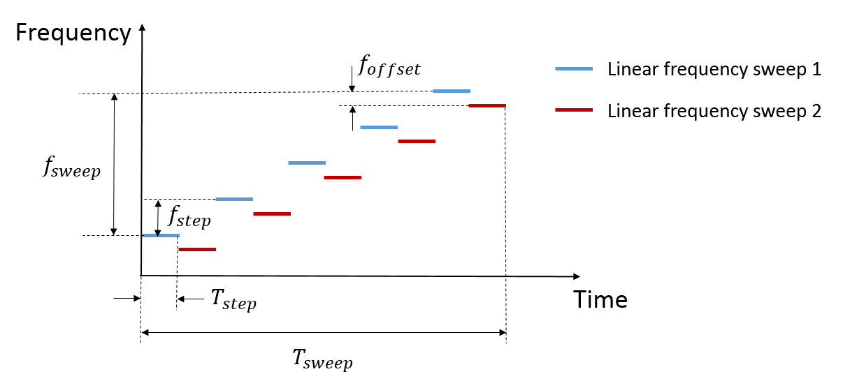
The figure indicates that the MFSK waveform is a combination of two linear FMCW waveforms with a fixed frequency offset. Unlike the regular FMCW waveforms, MFSK sweeps the entire bandwidth at discrete steps. Within each step, a single frequency continuous wave signal is transmitted. Because there are two tones within each step, it can be considered as a frequency shift keying (FSK) waveform. Thus, there is one set of range and Doppler relation from FMCW waveform and another set of range and Doppler relation from FSK. Combining two sets of relations together can help resolve the coupling between range and Doppler regardless of the number of targets present in the scene.
The following sections simulate the previous example, but use an MFSK waveform instead.
End-to-end Radar System Simulation Using MFSK Waveform
First, parameterize the MFSK waveform to satisfy the system requirement specified in [1]. Because the range resolution is 1 m, the sweep bandwidth is set at 150 MHz. In addition, the frequency offset is set at —294 kHz as specified in [1]. Each step lasts about 2 microseconds and the entire sweep has 1024 steps. Thus, each FMCW sweep takes 512 steps and the total sweep time is a little over 2 ms. Note that the sweep time is comparable to the FMCW signal used in previous sections.
mfskwaveform = phased.MFSKWaveform( ...
    'SampleRate',151e6, ...
    'SweepBandwidth',150e6, ...
    'StepTime',2e-6, ...
    'StepsPerSweep',1024, ...
    'FrequencyOffset',-294e3, ...
    'OutputFormat','Sweeps', ...
    'NumSweeps',1);
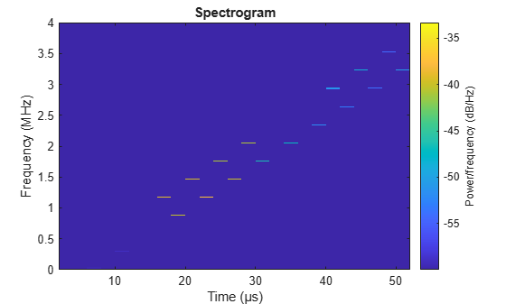
The figure below shows the spectrogram of the waveform. It is zoomed into a small interval to better reveal the time-frequency characteristics of the waveform.
numsamp_step = round(mfskwaveform.SampleRate*mfskwaveform.StepTime);
sig_display = mfskwaveform();
spectrogram(sig_display(1:8192),kaiser(3*numsamp_step,100), ...
    ceil(2*numsamp_step),linspace(0,4e6,2048),mfskwaveform.SampleRate, ...
    'yaxis','reassigned','minthreshold',-60)
Next, simulate the return of the system. Again, only one sweep is needed to estimate the range and Doppler.
Nsweep = 1;
release(channel);
channel.SampleRate = mfskwaveform.SampleRate;
release(receiver);
receiver.SampleRate = mfskwaveform.SampleRate;
xr = helperFMCWSimulate(Nsweep,mfskwaveform,sensormotion,tgtmotion, ...
    transmitter,channel,target,receiver);
The subsequent processing samples the return echo at the end of each step and group the sampled signals into two sequences corresponding to two sweeps. Note that the sampling frequency of the resulting sequence is now proportional to the time at each step, which is much less compared the original sample rate.
x_dechirp = reshape(xr(numsamp_step:numsamp_step:end),2,[]).';
fs_dechirp = 1/(2*mfskwaveform.StepTime);
As in the case of FMCW signals, the MFSK waveform is processed in the frequency domain. The following figures show the frequency spectrums of the received echoes corresponding to the two sweeps.
xf_dechirp = fft(x_dechirp);
num_xf_samp = size(xf_dechirp,1);
beatfreq_vec = (0:num_xf_samp-1).'/num_xf_samp*fs_dechirp;
clf
subplot(211),plot(beatfreq_vec/1e3,abs(xf_dechirp(:,1)))
grid on
ylabel('Magnitude')
title('Frequency spectrum for sweep 1')
subplot(212),plot(beatfreq_vec/1e3,abs(xf_dechirp(:,2)))
grid on
ylabel('Magnitude')
title('Frequency spectrum for sweep 2')
xlabel('Frequency (kHz)')
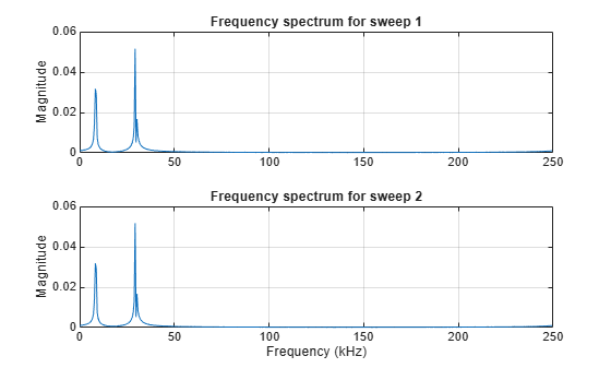
Note that there are two peaks in each frequency spectrum indicating two targets. In addition, the peaks are at the same locations in both returns so there are no ghost targets.
To detect the peaks, one can use a CFAR detector. Once detected, the beat frequencies as well as the phase differences between two spectra are computed at the peak locations.
cfar = phased.CFARDetector('ProbabilityFalseAlarm',1e-2, ...
    'NumTrainingCells',8);
peakidx = cfar(abs(xf_dechirp(:,1)),1:num_xf_samp);
Fbeat = beatfreq_vec(peakidx);
phi = angle(xf_dechirp(peakidx,2))-angle(xf_dechirp(peakidx,1));
Finally, the beat frequencies and phase differences are used to estimate the range and speed. Depending on how you construct the phase difference, the equations are slightly different. For the approach shown in this example, it can be shown that the range and speed satisfy the following relation:
where is the beat frequency, is the phase difference, is the wavelength, is the propagation speed, is the step time, is the frequency offset, is the sweep slope, is the range, and is the speed. Based on the equation, the range and speed are estimated as follows.
sweep_slope = mfskwaveform.SweepBandwidth/ ...
    (mfskwaveform.StepsPerSweep*mfskwaveform.StepTime);
temp = ...
    [-2/lambda 2*sweep_slope/c;-2/lambda*mfskwaveform.StepTime 2*mfskwaveform.FrequencyOffset/c]\ ...
    [Fbeat phi/(2*pi)].';
r_est = temp(2,:)
r_est = 1×2

   54.8564   49.6452
v_est = temp(1,:)
v_est = 1×2

   36.0089   -9.8495
The estimated range and speed match the true range and speed values very well.
Car: r = 50 m, v = -10 m/s
Truck: r = 55 m, v = 36 m/s
Summary
This example shows two simultaneous range and speed estimation approaches, using either a triangle sweep FMCW waveform or an MFSK waveform. This example shows that the MFSK waveform has an advantage over the FMCW waveform when multiple targets are present because it does not introduce ghost targets during the processing.
References
[1] Rohling, H. and M. Meinecke. Waveform Design Principle for Automotive Radar Systems, Proceedings of CIE International Conference on Radar, 2001.
You can also select a web site from the following list:
Americas
- América Latina (Español)
- Canada (English)
- United States (English)
Europe
- Belgium (English)
- Denmark (English)
- Deutschland (Deutsch)
- España (Español)
- Finland (English)
- France (Français)
- Ireland (English)
- Italia (Italiano)
- Luxembourg (English)
- Netherlands (English)
- Norway (English)
- Österreich (Deutsch)
- Portugal (English)
- Sweden (English)
- Switzerland
- United Kingdom (English)