Signal Detection Using Multiple Samples
This example shows how to detect a signal in complex, white Gaussian noise using multiple received signal samples. A matched filter is used to take advantage of the processing gain.
Introduction
The example, Signal Detection in White Gaussian Noise, introduces a basic signal detection problem. In that example, only one sample of the received signal is used to perform the detection. This example involves more samples in the detection process to improve the detection performance.
As in the previous example, assume that the signal power is 1 and the single sample signal to noise ratio (SNR) is 3 dB. The number of Monte Carlo trials is 100000. The desired probability of false alarm (Pfa) level is 0.001.
Ntrial = 1e5;             % number of Monte Carlo trials
Pfa = 1e-3;               % Pfa

snrdb = 3;                % SNR in dB
snr = db2pow(snrdb);      % SNR in linear scale
npower = 1/snr;           % noise power
namp = sqrt(npower/2);    % noise amplitude in each channel
Signal Detection Using Longer Waveform
As discussed in the previous example, the threshold is determined based on Pfa. Therefore, as long as the threshold is chosen, the Pfa is fixed, and vice versa. Meanwhile, one certainly prefers to have a higher probability of detection (Pd). One way to achieve that is to use multiple samples to perform the detection. For example, in the previous case, the SNR at a single sample is 3 dB. If one can use multiple samples, then the matched filter can produce an extra gain in SNR and thus improve the performance. In practice, one can use a longer waveform to achieve this gain. In the case of discrete time signal processing, multiple samples can also be obtained by increasing the sampling frequency.
Assume that the waveform is now formed with two samples:
Nsamp = 2;
wf = ones(Nsamp,1);
mf = conj(wf(end:-1:1));  % matched filter
For a coherent receiver, the signal, noise and threshold are given by
% fix the random number generator
rstream = RandStream.create('mt19937ar','seed',2009);

s = wf*ones(1,Ntrial);
n = namp*(randn(rstream,Nsamp,Ntrial)+1i*randn(rstream,Nsamp,Ntrial));
snrthreshold = db2pow(npwgnthresh(Pfa, 1,'coherent'));
mfgain = mf'*mf;
threshold = sqrt(npower*mfgain*snrthreshold);   % Final threshold T
If the target is present
x = s + n;
y = mf'*x;
z = real(y);
Pd = sum(z>threshold)/Ntrial
Pd = 0.3947
If the target is absent
x = n;
y = mf'*x;
z = real(y);
Pfa = sum(z>threshold)/Ntrial
Pfa = 0.0011
Notice that the SNR is improved by the matched filter.
snr_new = snr*mf'*mf;
snrdb_new = pow2db(snr_new)
snrdb_new = 6.0103
Plot the ROC curve with this new SNR value.
rocsnr(snrdb_new,'SignalType','NonfluctuatingCoherent','MinPfa',1e-4);
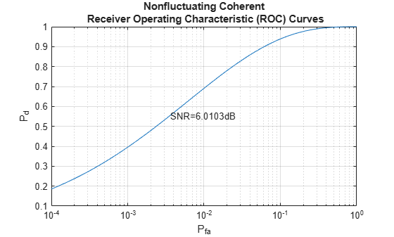
One can see from the figure that the point given by Pfa and Pd falls right on the curve. Therefore, the SNR corresponding to the ROC curve is the SNR of a single sample at the output of the matched filter. This shows that, although one can use multiple samples to perform the detection, the single sample threshold in SNR (snrthreshold in the program) does not change compared to the simple sample case. There is no change because the threshold value is essentially determined by Pfa. However, the final threshold, T, does change because of the extra matched filter gain. The resulting Pfa remains the same compared to the case where only one sample is used to do the detection. However, the extra matched gain improved the Pd from 0.1390 to 0.3947.
One can run similar cases for the noncoherent receiver to verify the relation among Pd, Pfa and SNR.
Signal Detection Using Pulse Integration
Radar and sonar applications frequently use pulse integration to further improve the detection performance. If the receiver is coherent, the pulse integration is just adding real parts of the matched filtered pulses. Thus, the SNR improvement is linear when one uses the coherent receiver. If one integrates 10 pulses, then the SNR is improved 10 times. For a noncoherent receiver, the relationship is not that simple. The following example shows the use of pulse integration with a noncoherent receiver.
Assume an integration of 2 pulses. Then, construct the received signal and apply the matched filter to it.
PulseIntNum = 2;
Ntotal = PulseIntNum*Ntrial;
s = wf*exp(1i*2*pi*rand(rstream,1,Ntotal));  % noncoherent
n = sqrt(npower/2)*...
    (randn(rstream,Nsamp,Ntotal)+1i*randn(rstream,Nsamp,Ntotal));
If the target is present
x = s + n;
y = mf'*x;
y = reshape(y,Ntrial,PulseIntNum);  % reshape to align pulses in columns
One can integrate the pulses using either of two possible approaches. Both approaches are related to the approximation of the modified Bessel function of the first kind, which is encountered in modeling the likelihood ratio test (LRT) of the noncoherent detection process using multiple pulses. The first approach is to sum abs(y)^2 across the pulses, which is often referred to as a square law detector. The second approach is to sum together abs(y) from all pulses, which is often referred to as a linear detector. For small SNR, square law detector is preferred while for large SNR, using linear detector is advantageous. We use square law detector in this simulation. However, the difference between the two kinds of detectors is normally within 0.2 dB.
For this example, choose the square law detector, which is more popular than the linear detector. To perform the square law detector, one can use the pulsint function. The function treats each column of the input data matrix as an individual pulse. The pulsint function performs the operation of
z = pulsint(y,'noncoherent');The relation between the threshold T and the Pfa, given this new sufficient statistics, z, is given by
where
is Pearson's form of the incomplete gamma function and L is the number of pulses used for pulse integration. Using a square law detector, one can calculate the SNR threshold involving the pulse integration using the npwgnthresh function as before.
snrthreshold = db2pow(npwgnthresh(Pfa,PulseIntNum,'noncoherent'));The resulting threshold for the sufficient statistics, z, is given by
mfgain = mf'*mf;
threshold = sqrt(npower*mfgain*snrthreshold);
The probability of detection is obtained by
Pd = sum(z>threshold)/Ntrial
Pd = 0.5343
Then, calculate the Pfa when the received signal is noise only using the noncoherent detector with 2 pulses integrated.
x = n;
y = mf'*x;
y = reshape(y,Ntrial,PulseIntNum);
z = pulsint(y,'noncoherent');
Pfa = sum(z>threshold)/Ntrial
Pfa = 0.0011
To plot the ROC curve with pulse integration, one has to specify the number of pulses used in integration in rocsnr function:
rocsnr(snrdb_new,'SignalType','NonfluctuatingNoncoherent',...
    'MinPfa',1e-4,'NumPulses',PulseIntNum);
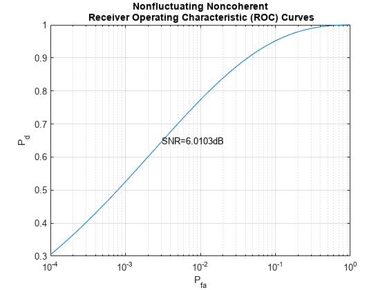
Again, the point given by Pfa and Pd falls on the curve. Thus, the SNR in the ROC curve specifies the SNR of a single sample used for the detection from one pulse.
Such an SNR value can also be obtained from Pd and Pfa using Albersheim's equation. The result obtained from Albersheim's equation is just an approximation, but is fairly good over frequently used Pfa, Pd and pulse integration range.
Note: Albersheim's equation has many assumptions, such as the target is nonfluctuating (Swirling case 0 or 5), the noise is complex, white Gaussian, the receiver is noncoherent and the linear detector is used for detection (square law detector for nonfluctuating target is also ok).
To calculate the necessary single sample SNR to achieve a certain Pd and Pfa, use the Albersheim function as
snr_required = albersheim(Pd,Pfa,PulseIntNum)
snr_required = 6.0009
This calculated required SNR value matches the new SNR value of 6 dB.
To see the improvement achieved in Pd by pulse integration, plot the ROC curve when there is no pulse integration used.
rocsnr(snrdb_new,'SignalType','NonfluctuatingNoncoherent',...
    'MinPfa',1e-4,'NumPulses',1);
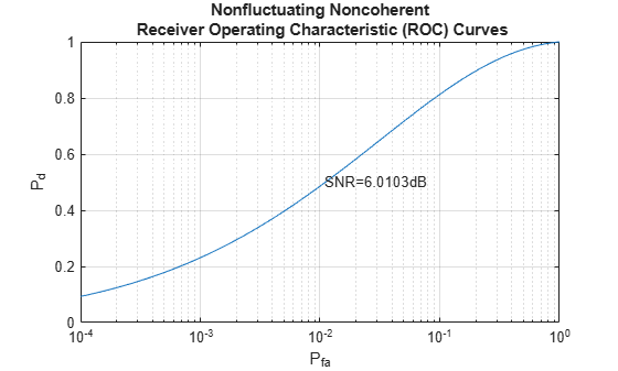
From the figure, one can see that without pulse integration, Pd can only be around 0.24 with Pfa at 1e-3. With 2-pulse integration, as illustrated in the above Monte Carlo simulation, for the same Pfa, the Pd is around 0.53.
Summary
This example showed how using multiple signal sample in detection can improve the probability of detection while maintaining a desired probability of false alarm level. In particular, it showed using either longer waveform or pulse integration technique to improve Pd. The example illustrates the relation among Pd, Pfa, ROC curve and Albersheim's equation. The performance is calculated using Monte Carlo simulations.
You can also select a web site from the following list:
Americas
- América Latina (Español)
- Canada (English)
- United States (English)
Europe
- Belgium (English)
- Denmark (English)
- Deutschland (Deutsch)
- España (Español)
- Finland (English)
- France (Français)
- Ireland (English)
- Italia (Italiano)
- Luxembourg (English)
- Netherlands (English)
- Norway (English)
- Österreich (Deutsch)
- Portugal (English)
- Sweden (English)
- Switzerland
- United Kingdom (English)