Modeling Perturbations and Element Failures in a Sensor Array
This example shows how to model amplitude, phase, position and pattern perturbations as well as element failures in a sensor array.
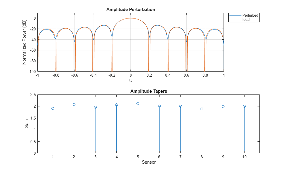
Amplitude Perturbation
This section shows how to add gain or amplitude perturbations on a uniform linear array (ULA) of 10 elements. Consider the perturbations to be statistically independent zero-mean Gaussian random variables with standard deviation of 0.1.
Create a ULA antenna of 10 elements.
N = 10;
ula = phased.ULA(N);
Create amplitude or gain perturbations on the array
rs = rng(7);
pertStDev = 0.1;

perturbations(ula,'TaperMagnitude','Normal',1,pertStDev);
perturbedULA = perturbedArray(ula);
Compare the response of the perturbed to the ideal array.
% Overlay responses
c = 3e8; freq = c;

subplot(2,1,1);
helperCompareResponses(perturbedULA,ula,'Amplitude Perturbation', ...
                       {'Perturbed','Ideal'});

% Show the corresponding tapers
subplot(2,1,2);
stem(perturbedULA.Taper)
title('Amplitude Tapers');xlabel('Sensor');ylabel('Gain');
Phase Perturbation
This section shows how to add phase perturbations to the ULA antenna used in the previous section. Consider the perturbations distribution to be similar to the previous section.
perturbations(ula,'TaperMagnitude','none');
perturbations(ula,'TaperPhase','Normal',0,pertStDev);
perturbedULA = perturbedArray(ula);
Compare the response of the perturbed to the ideal array.
% Overlay responses
subplot(2,1,1);
helperCompareResponses(perturbedULA,ula,'Phase Perturbation', ...
                       {'Perturbed','Ideal'});

% Show the corresponding tapers
subplot(2,1,2);
stem(angle(perturbedULA.Taper))
title('Phase Tapers');xlabel('Sensor');ylabel('Phase (rad)');
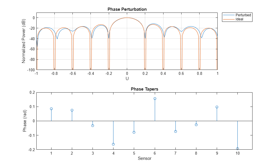
Notice how the perturbed response has shallower nulls.
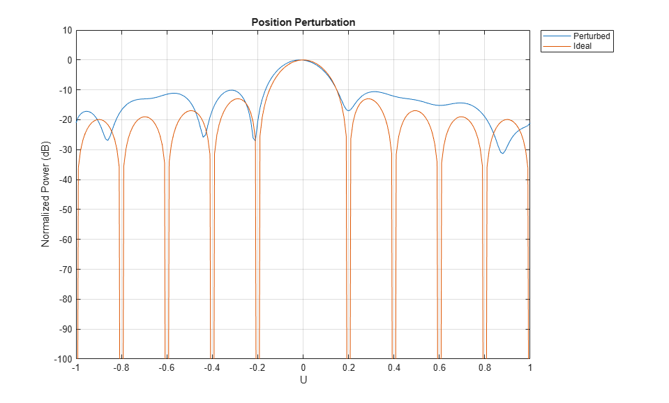
Position Perturbation
This section shows how to perturb the positions of the ULA sensor along the three axes.
perturbations(ula,'TaperPhase','none');
perturbations(ula,'ElementPosition','Normal',0,pertStDev);
perturbedULA = perturbedArray(ula);
Compare the response of the perturbed to the ideal array.
% Overlay responses
clf;
helperCompareResponses(perturbedULA,phased.ULA(N), ...
    'Position Perturbation', {'Perturbed','Ideal'});
View the array.
viewArray(perturbedULA);
title('Element Positions');

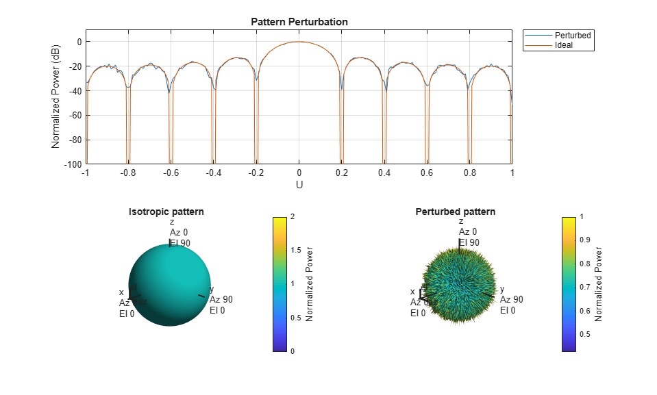
Pattern Perturbation
This section will replace the isotropic antenna elements with perturbed patterns.
First create 10 custom antenna elements with perturbed isotropic patterns.
antenna = phased.CustomAntennaElement;
radpat = antenna.MagnitudePattern;
element = cell(1,N);
for i = 1:N
    perturbedAntenna = clone(antenna);
    perturbedAntenna.MagnitudePattern = ...
        pow2db(1+randn(size(radpat))*pertStDev);
    element{i} = perturbedAntenna;
end
Here, map the 10 patterns in the cell array 'element' to the 10 sensors using the ElementIndices property.
perturbedULA = phased.HeterogeneousULA('ElementSet',element, ...
                                        'ElementIndices',1:N);
Compare the response of the perturbed to the ideal array.
% Overlay responses
clf;
subplot(2,2,[1 2]);
helperCompareResponses(perturbedULA,phased.ULA(N),...
    'Pattern Perturbation', ...
    {'Perturbed','Ideal'});

% Show the perturbed pattern response next to the ideal isotropic pattern
subplot(2,2,3);
pattern(ula.Element,freq,'CoordinateSystem','polar','Type','power')
title('Isotropic pattern');
subplot(2,2,4);
pattern(element{1},freq,'CoordinateSystem','polar','Type','power')
title('Perturbed pattern');
Element Failures
This section will model element failures on an 8 by 10 uniformly rectangular array. Each element has 10 percent probability of failing.
Create a URA antenna of 8 by 10 elements.
ura = phased.URA([8 10]);
Failures can be modeled by setting the gain on the corresponding sensor to 0. Here a matrix is created in which each element has a 10 percent probability of being 0.
perturbations(ura,'ElementFailure','RandomFail',0.1);
perturbedURA = perturbedArray(ura);

% ura.Taper  = double(rand(8,10) > .1);
Compare the response of the array with failed elements to the ideal array.
% Overlay responses
clf;
helperCompareResponses(perturbedURA,ura,'Element Failures', ...
                       {'Failures','No Failures'});
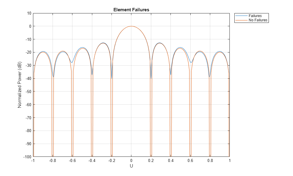
Notice how deep nulls are hard to attain in the response of the array with failed elements.
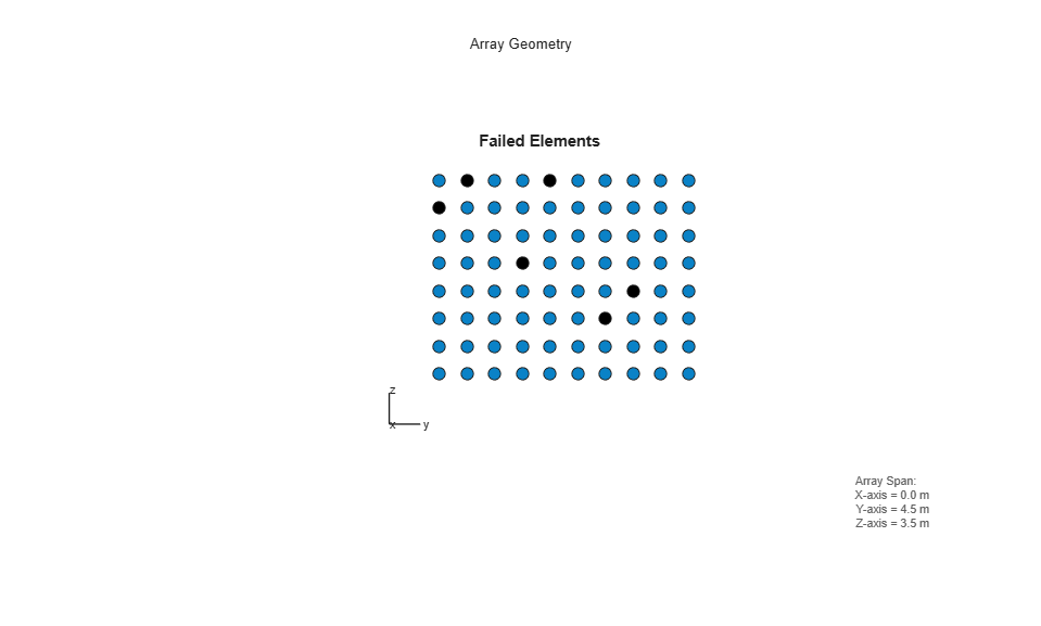
View the failed elements.
viewArray(perturbedURA,'ShowTaper',true);
title('Failed Elements');

% reset the random seed
rng(rs)
Summary
This example showed how to model different kind of perturbations as well as element failures. It also demonstrated the effect on the array response for all the cases.
You can also select a web site from the following list:
Americas
- América Latina (Español)
- Canada (English)
- United States (English)
Europe
- Belgium (English)
- Denmark (English)
- Deutschland (Deutsch)
- España (Español)
- Finland (English)
- France (Français)
- Ireland (English)
- Italia (Italiano)
- Luxembourg (English)
- Netherlands (English)
- Norway (English)
- Österreich (Deutsch)
- Portugal (English)
- Sweden (English)
- Switzerland
- United Kingdom (English)