Array Pattern Synthesis Part I: Nulling, Windowing, and Thinning
This example shows how to use Phased Array System Toolbox™ to solve some array synthesis problems.
In phased array design applications, it is often necessary to find a way to taper element responses so that the resulting array pattern satisfies certain performance criteria. Typical performance criteria include the mainlobe location, null location(s) and sidelobe levels.
Interference Removal Using Sidelobe Canceller
A common requirement when synthesizing beam patterns is pointing a null towards a given arrival direction. This helps suppress interference from that direction and improves the signal-to-interference ratio. The interference is not always malicious- an airport radar system may need to suppress interference from a nearby radio station. In this case, the position of the radio station is known and a sidelobe cancellation algorithm can be used to remove the interference.
Sidelobe cancellation is useful for suppressing interference that enters through the array's sidelobes. In this case, because the interference direction is known, the algorithm is simple. Form a beam that points towards the interference direction, then scale the beam weights and subtract scaled weights from the weights for the beam patterns that point towards any other look direction. This process always places a strong null in the interference direction.
The following example shows how to design the weights of the radar so that it scans between -30 and 30 degrees yet always keeps a null at 40 degrees. Assume that the radar uses a 10-element ULA that is parallel to the ground and that the known radio interference arrives from 40 degrees azimuth.
c = 3e8;        % signal propagation speed
fc = 1e9;       % signal carrier frequency
lambda = c/fc;  % wavelength

thetaad = -30:5:30;     % look directions
thetaan = 40;           % interference direction

ula = phased.ULA(10,lambda/2);
ula.Element.BackBaffled = true;

% Calculate the steering vector for null directions
wn = steervec(getElementPosition(ula)/lambda,thetaan);

% Calculate the steering vectors for lookout directions
wd = steervec(getElementPosition(ula)/lambda,thetaad);

% Compute the response of desired steering at null direction
rn = wn'*wd/(wn'*wn);

% Sidelobe canceler - remove the response at null direction
w = wd-wn*rn;

% Plot the pattern
pattern(ula,fc,-180:180,0,'PropagationSpeed',c,'Type','powerdb',...
    'CoordinateSystem','rectangular','Weights',w);
hold on; legend off;
plot([40 40],[-100 0],'r--','LineWidth',2)
text(40.5,-5,'\leftarrow Interference Direction','Interpreter','tex',...
    'Color','r','FontSize',10)
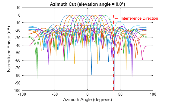
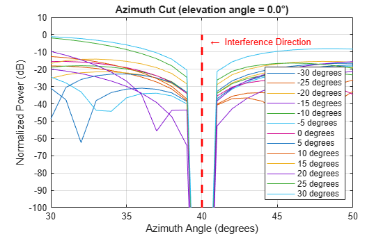
The figure above shows the resulting beam patterns for look directions from -30 degrees azimuth to 30 degrees azimuth, in 5 degrees increment. It is clear from the zoomed figure below that no matter where the look direction is, the radar beam pattern has a strong null at the interference direction.
% Zoom
xlim([30 50])
legend(arrayfun(@(k)sprintf('%d degrees',k),thetaad,...
    'UniformOutput',false),'Location','SouthEast');
Pattern Synthesis Using Windowing Function
Another frequent problem when designing a phased array is matching a desired beam pattern to a specification that is handed to you. Often, the requirements are expressed in terms of beamwidth and sidelobe level.
The process of addressing such a problem often includes these steps:
Observe the desired pattern and decide an array geometry;
Choose an array size based on the desired beamwidth;
Design tapers based on the desired sidelobe level;
Iterate on adjusting the parameter obtained step 2 and 3 to get a best match.
The following example illustrates these four steps. First, observe the desired pattern shown in the following figure.
load desiredSynthesizedAntenna;

clf;
pattern(mysteryAntenna,fc,'CoordinateSystem','polar','Type','powerdb');
view(50,20);
ax = gca;
ax.Position = [-0.15 0.1 0.9 0.8];
camva(4.5);
campos([520 -250 200]);
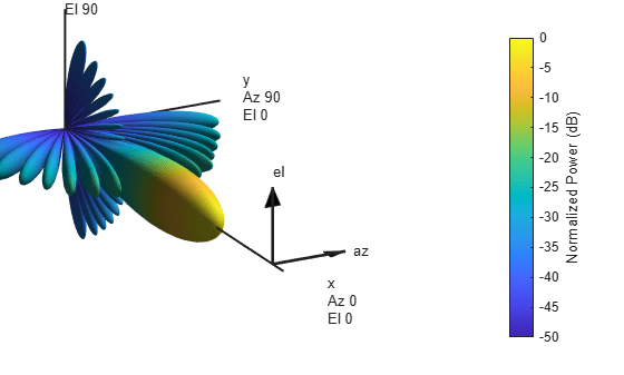
The 3D radiation patterns exhibits some symmetries in both azimuth and elevation cuts. Therefore, the pattern may be best obtained using a uniform rectangular array (URA). It is also clear from the plot that there is no energy radiated toward back of the array.
Next, determine the size of the array. To avoid grating lobes, the element spacing is set to half wavelength. For a URA, the sizes along the azimuth and elevation directions can be derived from the required beamwidths along azimuth and elevation directions, respectively. In the case of half wavelength spacing, the number of elements along a certain direction can be approximated by
where is the beamwidth along that direction. Hence, the aperture size of the URA can be computed as
[azpat,elpat,az,el] = helperExtractSynthesisPattern(mysteryAntenna,fc,c);

% Azimuth direction
idx = find(azpat>pow2db(1/2));
azco = [az(idx(1)) az(idx(end))]; % azimuth cutoff
N_col = round(2/sind(diff(azco)))
N_col = 19
% Elevation direction
idx = find(elpat>pow2db(1/2));
elco = [el(idx(1)) el(idx(end))]; % elevation cutoff
N_row = round(2/sind(diff(elco)))
N_row = 14
The estimation suggests to start with a 14x19 URA.
% Form the URA
ura = phased.URA([N_row N_col],[lambda/2 lambda/2]);
ura.Element.BackBaffled = true;
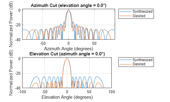
helperArraySynthesisComparison(ura,mysteryAntenna,fc,c)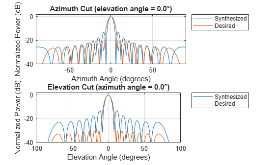
The figure shows that the synthesized array exceeds the beamwidth requirement of the desired pattern. However, the sidelobes are much larger than the desired pattern. You can reduce the sidelobes by applying a windowing operation to the array. Because the URA can be considered to be the combination of two separable uniform linear arrays (ULA), the window can be designed independently along both the azimuth and elevation directions using familiar filter design methods.
The code below shows how to obtain the windows for azimuth and elevation directions.
AzSidelobe = 20;
Ap = 0.1;                                % Passband ripples
AzWeights = designfilt('lowpassfir','FilterOrder',N_col-1,...
    'CutoffFrequency',azco(2)/90,'PassbandRipple',0.1,...
    'StopBandAttenuation',AzSidelobe);
azw = AzWeights.Coefficients;

ElSidelobe = 30;
ElWeights = designfilt('lowpassfir','FilterOrder',N_row-1,...
    'CutoffFrequency',elco(2)/90,'PassbandRipple',0.1,...
    'StopBandAttenuation',ElSidelobe);
elw = ElWeights.Coefficients;

% Assign the weights to the array
ura.Taper = elw(:)*azw(:).';

% Compare the pattern
helperArraySynthesisComparison(ura,mysteryAntenna,fc,c)
The figure shows that the resulting sidelobe level is lower compared to the previous design but still does not satisfy the requirement. By some trials and errors, the following parameters are used to create the final design:
N_row = N_row+2;        % trial and error
N_col = N_col-3;        % trial and error
AzSidelobe = 26;
ElSidelobe = 35;

AzWeights = designfilt('lowpassfir','FilterOrder',N_col-1,...
    'CutoffFrequency',azco(2)/90,'PassbandRipple',0.1,...
    'StopBandAttenuation',AzSidelobe);
azw = AzWeights.Coefficients;

ElWeights = designfilt('lowpassfir','FilterOrder',N_row-1,...
    'CutoffFrequency',elco(2)/90,'PassbandRipple',0.1,...
    'StopBandAttenuation',ElSidelobe);
elw = ElWeights.Coefficients;

ura = phased.URA([N_row N_col],[lambda/2 lambda/2]);
ura.Element.BackBaffled = true;

ura.Taper = elw(:)*azw(:).';

helperArraySynthesisComparison(ura,mysteryAntenna,fc,c)
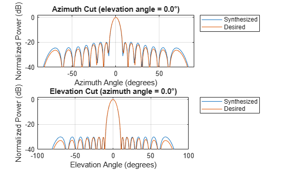
The figure shows that the beamwidth and sidelobe levels of the synthesized pattern match the desired specifications. The following figures show the desired 3D pattern, the synthesized 3D pattern, the resulting array geometry, and the taper.
helperArraySynthesisComparison(ura,mysteryAntenna,fc,c,'3d')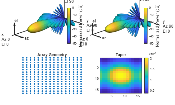
Array Thinning Using Genetic Algorithm
Many array synthesis problems can be treated as optimization problems, especially for arrays with large apertures or complex geometries. In those situations, a closed form solution often does not exist and the solution space is very large. For example, for a large array, it is often necessary to thin the array to control the sidelobe levels to avoid wasting power delivered to each antenna element. In this case, an element can be turned on or off. If you were to try all possible solutions in a 40x40 URA, you would need to try combinations, which is unrealistic. Optimization techniques are often adopted in this situation.
A frequently used optimization technique is the genetic algorithm. A genetic algorithm achieves an optimal solution by simulating the natural selection process. It starts with randomly selected candidates as the first generation. At each evolution cycle, the algorithm sorts the generation according to a predetermined performance measure (in the thinned array example, the performance measure would be the ratio of peak-to-sidelobe level), and then discards the ones with lower performance scores. The algorithm then mutates the remaining candidates to generate a newer generation and repeats the process, until it reaches a stop condition, such as the maximum number of generations.
The following example shows how to thin a 40x40 URA using the thinnedArray method. The thinnedArray method uses a genetic algorithm to minimize the total number of active array elements such that the resulting maximum sidelobe level is below a specified desired value.
Create a 40x40 URA of cosine antenna elements.
% Set the random number generator for reproducibility.
rng('default');

Nside = 40;
uraFull = phased.URA(Nside,lambda/2,"Element",phased.CosineAntennaElement);
Plot the beampattern of the full array.
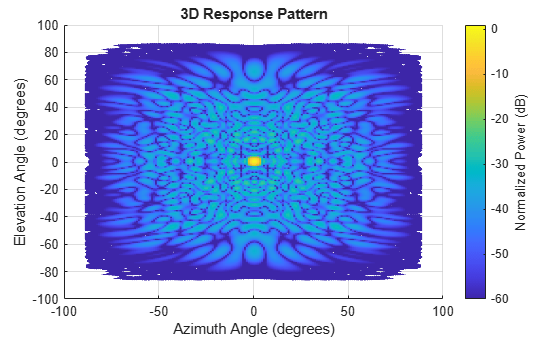
az = -90:90;            % Azimuth angles
el = -90:90;            % Elevation angles

figure
pattern(uraFull,fc,az,el,'Type','powerdb','CoordinateSystem','rectangular')
view(2)
clim([-60 1])
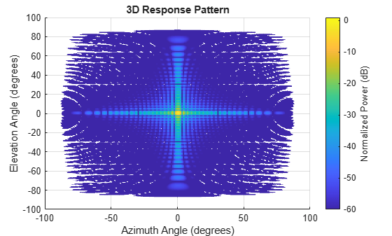
The sidelobe level of the full array is about 13.5dB. Use the thinnedArray method of the uraFull object to create a thinned array. Set the desired sidelobe level to -25 dB. Assume that the array is steered to the broadside.
sll = -25;              % Desired sidelobe level
[uraThin,w,info] = thinnedArray(uraFull,fc,[0; 0],sll);

figure
pattern(uraThin,fc,az,el,'Type','powerdb','CoordinateSystem','rectangular')
view(2)
clim([-60 1])
The thinnedArray method also returns a struct with information about the produced thinned array.
info
info = struct with fields:
      ThinningFactor: 45.7500
    MaxSidelobeLevel: -25.2907
    BeamwidthThinned: [2x1 double]
       BeamwidthFull: [2x1 double]
The reported thinning factor, the percentage of the array elements that remain active after thinning, is less than 50%. This means that more than half of the array elements are off. Compared to the full array, the resulting thinned array can save the cost of implementing T/R switches behind dummy elements, which in turn leads to a roughly 50% saving on the consumed power. Also note that even though the thinned array uses fewer elements, the beamwidth is close to what could be achieved with a full array.
info.BeamwidthFull
ans = 2×1

    2.5400
    2.5400
info.BeamwidthThinned
ans = 2×1

    3.1800
    3.1800
The MaxSidelobeLevel field reports the maximum sidelobe level achieved during the optimization. Although it is close to the desired sidelobe level, the genetic algorithm optimization does not guarantee that the sidelobe level constraint is going to be satisfied.
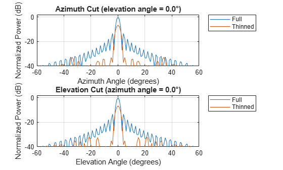
The thinnedArray method tries to achieve the desired sidelobe level over the entire azimuth-elevation space. Verify that the achieved sidelobe level along the azimuth and the elevation cuts is equal to or lower than the desired value.
clf
helperThinnedArrayComparison(uraFull,fc,c,[ones(Nside^2, 1) w(:)],...
    {'Full','Thinned'});
Display the geometry of the generated thinned array. The dummy elements are represented by black circles.
clf
viewArray(uraThin,'ShowTaper',true);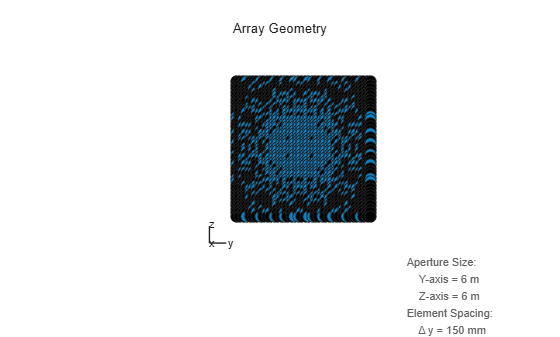
The maximum sidelobe level of the obtained thinned array is close to the desired value only when the array is steered to the broadside. If steered off broadside, the maximum sidelobe level will increase significantly.
Let the maximum scan angle be 45 degrees in azimuth and 30 degrees in elevation. Plot beampattern when the thinned array is pointing to the maximum scan angle.
steeringVector = phased.SteeringVector('SensorArray',uraFull);
maxScanAngle = [45; 30];
sv = steeringVector(fc, maxScanAngle);

figure;
pattern(uraThin,fc,az,el,'Type','powerdb','CoordinateSystem','rectangular',...
    'Weights',sv);
view(2)
clim([-60 1])

The maximum sidelobe level is now close to -16 dB.
To maintain a good sidelobe performance, the scanning array should be thinned when pointing to the maximum scan angle. Then the sidelobes for the smaller scan angles will be close to or even lower than the desired level.
[uraThinScan,~,info] = thinnedArray(uraFull,fc,maxScanAngle,sll);
info
info = struct with fields:
      ThinningFactor: 62.5000
    MaxSidelobeLevel: -21.9208
    BeamwidthThinned: [2x1 double]
       BeamwidthFull: [2x1 double]
The maximum sidelobe level when steered to the maximum scan angle is now around -22 dB. Plot the array beampattern when steered to the maximum scan angle, the broadside, and two positions in between. Note that the maximum sidelobe level is the highest when pointing to the maximum scan angle.
azel = [maxScanAngle [30 15 0; 20 10 0]];
sv = steeringVector(fc,azel);

figure
tiledlayout(2,2);

for i = 1:4
    nexttile;
    pattern(uraThinScan,fc,az,el,'Type','powerdb','CoordinateSystem','rectangular',...
        'Weights',sv(:, i));
    view(2)
    clim([-60 1])
    title(sprintf('Az = %.1f, El = %.1f',azel(1, i),azel(2, i)));
end

Array thinning can also be used to create null regions in the specific directions. Specify a null region as start and stop directions in azimuth and elevation.
nstart = [25; 15];      % Start position of the null region
nstop = [30; 18];       % Stop position of the null region
[uraThinNullSymmetric,~,info] = thinnedArray(uraFull,fc,[0;0],sll,nstart,nstop);
info
info = struct with fields:
        ThinningFactor: 49.2500
      MaxSidelobeLevel: -25.2999
    MinNullRegionDepth: -51.8854
      BeamwidthThinned: [2x1 double]
         BeamwidthFull: [2x1 double]
figure;
pattern(uraThinNullSymmetric,fc,az,el,'Type','powerdb','CoordinateSystem','rectangular');
rectangle('Position', [nstart(1) nstart(2) nstop(1)-nstart(1) nstop(2)-nstart(2)],...
    'EdgeColor','r');
view(2)
clim([-60 1])

The minimum null depth within the specified null region after thinning is reported in the MinNullRegionDepth field of the returned info struct.
The specified null region is shown on the beampattern by a red rectangle. Note that the same null region appears in the locations that are symmetric with respect to the azimuth and the elevation axis. This is because by default, the thinnedArray method exploits symmetry in both rows and columns of a URA to speed up the computation. Dividing the URA in four symmetric quarters allows for reducing the number of unknown thinning coefficients by four. This allows the underlying genetic algorithm to find a solution faster. To treat all array elements independently, set the 'SymmetricThinning' name-value pair to false when calling the thinnedArray method. In this case there will be only one additional null region symmetric with respect to the origin.
It is worth noting that the genetic algorithm does not always land on the same solution in each trial. However, in general the resulting beam patterns share a similar sidelobe level.
Summary
This example shows several approaches to perform array synthesis on a phased array. In practice, one needs to choose the appropriate synthesis method according to the specific constraint of the application, such as the size of the array aperture, the shape of the array geometry, etc.
Reference
[1] Randy L. Haupt, Thinned Arrays Using Genetic Algorithms, IEEE Transactions on Antennas and Propagation, Vol 42, No 7, 1994
[2] Randy L. Haupt, An Introduction to Genetic Algorithms for Electromagnetics, IEEE antennas and Propagation Magazine, Vol 37, No 2, 1995
[3] Harry L. Van Trees, Optimum Array Processing, Wiley-Interscience, 2002
You can also select a web site from the following list:
Americas
- América Latina (Español)
- Canada (English)
- United States (English)
Europe
- Belgium (English)
- Denmark (English)
- Deutschland (Deutsch)
- España (Español)
- Finland (English)
- France (Français)
- Ireland (English)
- Italia (Italiano)
- Luxembourg (English)
- Netherlands (English)
- Norway (English)
- Österreich (Deutsch)
- Portugal (English)
- Sweden (English)
- Switzerland
- United Kingdom (English)