Wave Equation on Square Domain

This example shows how to solve the wave equation using the solvepde function.

The standard second-order wave equation is

$$\frac{{\partial }^{2}u}{\partial t^2}-\nabla \cdot \nabla u=0.$$

To express this in toolbox form, note that the solvepde function solves problems of the form

$$m\frac{{\partial }^{2}u}{\partial t^2}-\nabla \cdot (c\nabla u)+au=f.$$

So the standard wave equation has coefficients $$m=1$$, $$c=1$$, $$a=0$$, and $$f=0$$.

c = 1;
a = 0;
f = 0;
m = 1;

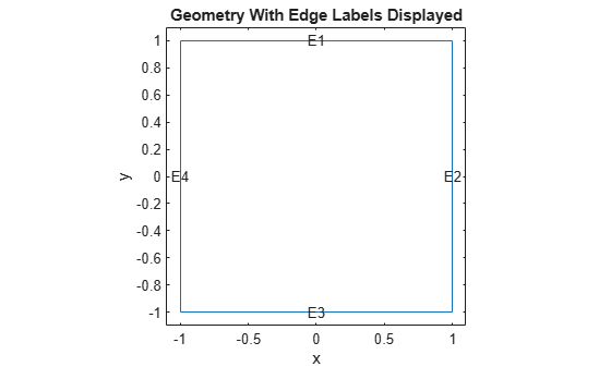
Solve the problem on a square domain. The squareg function describes this geometry. Create a model object and include the geometry. Plot the geometry and view the edge labels.

numberOfPDE = 1;
model = createpde(numberOfPDE);
geometryFromEdges(model,@squareg);
pdegplot(model,"EdgeLabels","on"); 
ylim([-1.1 1.1]);
axis equal
title("Geometry With Edge Labels Displayed")
xlabel("x")
ylabel("y")

Specify PDE coefficients.

specifyCoefficients(model,"m",m,"d",0,"c",c,"a",a,"f",f);

Set zero Dirichlet boundary conditions on the left (edge 4) and right (edge 2) and zero Neumann boundary conditions on the top (edge 1) and bottom (edge 3).

applyBoundaryCondition(model,"dirichlet","Edge",[2,4],"u",0);
applyBoundaryCondition(model,"neumann","Edge",([1 3]),"g",0);

Create and view a finite element mesh for the problem.

generateMesh(model);
figure
pdemesh(model);
ylim([-1.1 1.1]);
axis equal
xlabel x
ylabel y

Set the following initial conditions:

• $$u(x,0)=\arctan \left(\cos \left(\frac{\pi x}{2}\right)\right)$$.

• $${\frac{\partial u}{\partial t}|}_{t=0}=3\sin (\pi x)\exp \left(\sin \left(\frac{\pi y}{2}\right)\right)$$.

u0 = @(location) atan(cos(pi/2*location.x));
ut0 = @(location) 3*sin(pi*location.x).*exp(sin(pi/2*location.y));
setInitialConditions(model,u0,ut0);

This choice avoids putting energy into the higher vibration modes and permits a reasonable time step size.

Specify the solution times as 31 equally-spaced points in time from 0 to 5.

n = 31;
tlist = linspace(0,5,n);

Set the SolverOptions.ReportStatistics of model to 'on'.

model.SolverOptions.ReportStatistics ='on';
result = solvepde(model,tlist);

441 successful steps
34 failed attempts
952 function evaluations
1 partial derivatives
115 LU decompositions
951 solutions of linear systems

u = result.NodalSolution;

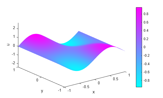
Create an animation to visualize the solution for all time steps. Keep a fixed vertical scale by first calculating the maximum and minimum values of u over all times, and scale all plots to use those $$z$$-axis limits.

figure
umax = max(max(u));
umin = min(min(u));
for i = 1:n
    pdeplot(model,"XYData",u(:,i),"ZData",u(:,i), ...
                  "ZStyle","continuous","Mesh","off");
    axis([-1 1 -1 1 umin umax]); 
    caxis([umin umax]);
    xlabel x
    ylabel y
    zlabel u
    M(i) = getframe;
end

To play the animation, use the movie(M) command.

×

Open Example

You have a modified version of this example. Do you want to open this example with your edits?

No, overwrite the modified version Yes