von Mises Effective Stress and Displacements: PDE Modeler App
This example shows how to compute the displacements u and v and the von Mises effective stress for a steel plate that is clamped along a right-angle inset at the lower-left corner, and pulled along a rounded cut at the upper-right corner. The example uses the PDE Modeler app. The app also lets you compute and visualize other properties, such as the x- and y-direction strains and stresses and the shear stress.
Consider a steel plate that is clamped along a right-angle inset at the lower-left corner, and pulled along a rounded cut at the upper-right corner. All other sides are free. The steel plate has the following properties:
Dimensions 1 m-by-1 m-by 0.001 m;
Inset is 1/3-by-1/3 m
The rounded cut runs from (2/3, 1) to (1, 2/3)
Young's modulus: 196 · 103 (MN/m2)
Poisson's ratio: 0.31.
The curved boundary is subjected to an outward normal load of 500 N/m. To specify a surface traction, divide the load by the thickness (0.001 m). Thus, the surface traction is 0.5 MN/m2. The force unit in this example is MN.
To solve this problem in the PDE Modeler app, follow these steps:
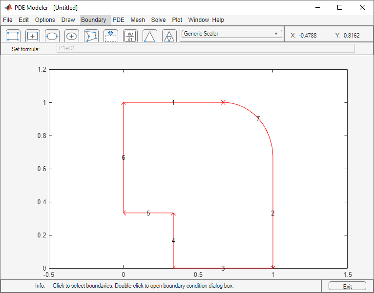
Draw a polygon with corners (0 1), (2/3,1), (1,2/3), (1,0), (1/3,0), (1/3,1/3), (0,1/3) and a circle with the center (2/3, 2/3) and radius 1/3.
pdepoly([0 2/3 1 1 1/3 1/3 0],[1 1 2/3 0 0 1/3 1/3])
pdecirc(2/3,2/3,1/3)
Set the x-axis limit to
[-0.5 1.5]and y-axis limit to[0 1.2]. To do this, select Options > Axes Limits and set the corresponding ranges.Model the geometry by entering
P1+C1in the Set formula field.Set the application mode to Structural Mechanics, Plane Stress.
Remove all subdomain borders. To do this, switch to the boundary mode by selecting Boundary > Boundary Mode. Then select Boundary > Remove All Subdomain Borders.
Display the edge labels by selecting Boundary > Show Edge Labels.
Specify the boundary conditions. To do this, select Boundary > Specify Boundary Conditions.
For convenience, first specify the Neumann boundary condition
g1 = g2 = 0,q11 = q12 = q21 = q22 = 0(no normal stress) for all boundaries. Use Edit > Select All to select all boundaries.For the two clamped boundaries at the inset in the lower left (edges 4 and 5), specify the Dirichlet boundary condition with zero displacements:
h11 = 1,h12 = 0,h21 = 0,h22 = 1,r1 = 0,r2 = 0. Use Shift+click to select several boundaries.For the rounded cut (edge 7), specify the Neumann boundary condition:
g1 = 0.5*nx,g2 = 0.5*ny,q11 = q12 = q21 = q22 = 0.
Specify the coefficients by selecting PDE > PDE Specification or clicking the
 button on the toolbar. Specify
 E = 196E3andnu = 0.31. The material is homogeneous, so the same valuesEandnuapply to the entire 2-D domain. Because there are no volume forces, specifyKx = Ky = 0. The elliptic type of PDE for plane stress does not use density, so you can specify any value. For example, specifypho = 0.Initialize the mesh by selecting Mesh > Initialize Mesh. Refine the mesh by selecting Mesh > Refine Mesh.
Refining the mesh in areas where the gradient of the solution (the stress) is large. To do this, select Solve > Parameters. In the resulting dialog box, select Adaptive mode. Use the default adaptation options: the Worst triangles triangle selection method with the Worst triangle fraction set to
0.5.Solve the PDE by selecting Solve > Solve PDE or clicking the
 button on the toolbar.
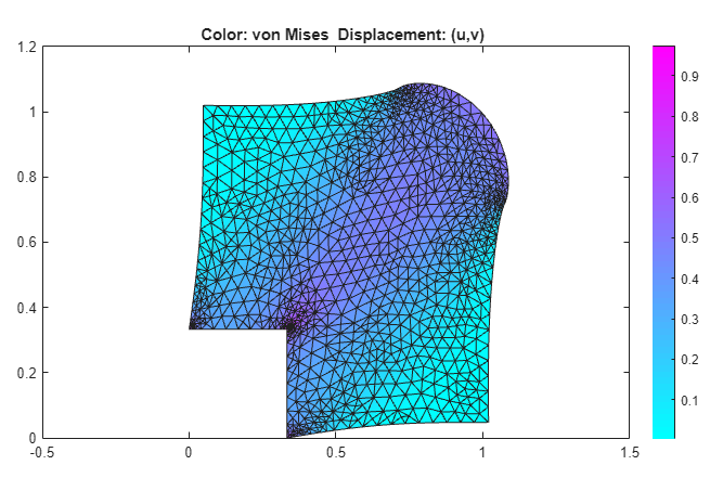
Plot the von Mises effective stress using color. Plot the displacement vector field (u,v) using a deformed mesh. To do this:
Select Plot > Parameters.
In the resulting dialog box, select the Color and Deformed mesh options. Select
von
                            Mises
from the Color drop-down menu. Select Show Mesh to observe the refined mesh in large stress areas.
By selecting other options from the Color drop-down menu, you can visualize different strain and stress properties, such as the x- and y-direction strains and stresses, the shear stress, and the principal stresses and strains. You also can plot combinations of scalar and vector properties by using color, height, vector field arrows, and displacements in a 3-D plot to represent different properties.