Skin Effect in Copper Wire with Circular Cross Section: PDE Modeler App
This example shows the skin effect when a wire with a circular cross section carries AC current. In a solid conductor, such as the wire, AC current travels near the surface of a wire and avoids the area close to the center of the wire. This effect is called the skin effect. The example uses the PDE Modeler app.
The Helmholtz equation
describes the propagation of plane electromagnetic waves in imperfect dielectrics and good conductors (σ » ωε). The coefficient of dielectricity is ε = 8.8*10-12 F/m. The conductivity of copper is σ = 57 * 106 S/m. The magnetic permeability of copper is close to the magnetic permeability of a vacuum, µ = 4π*10–7 H/m. The ω2ε-term is negligible at the line frequency (50 Hz).
Due to induction, the current density in the interior of the conductor is smaller than at the outer surface, where it is set to JS = 1. The Dirichlet condition for the electric field is Ec = 1/σ. In this case, the analytical solution is
Here,
R is the radius of the wire, r is the distance from the center line, and J0(x) is the first Bessel function of zeroth order.
To solve this problem in the PDE Modeler app, follow these steps:
Draw a circle with a radius of 0.1. The circle represents a cross section of the conductor.
pdecirc(0,0.05,0.1)
Set the x-axis limit to
[-0.2 0.2]and the y-axis limit to[-0.1 0.2]. To do this, select Options > Axes Limits and set the corresponding ranges. Then select Options > Axes Equal.Set the application mode to AC Power Electromagnetics.
Specify the Dirichlet boundary condition E = JS/σ = 1/σ for the boundary of the circle. To do this:
Switch to the boundary mode by selecting Boundary > Boundary Mode.
Select all boundaries by using Edit > Select All.
Select Boundary > Specify Boundary Conditions.
Specify
h = 1andr = 1/57E6.
Specify the PDE coefficients. To do this, switch to the PDE mode by selecting PDE > PDE Mode. Then select PDE > PDE Specification or click the
 button on the toolbar. Specify the following
values:
button on the toolbar. Specify the following
values:Angular frequency
omega = 2*pi*50Magnetic permeability
mu = 4*pi*1E-7Conductivity
sigma = 57E6Coefficient of dielectricity
epsilon = 8.8E-12
Initialize the mesh by selecting Mesh > Initialize Mesh.
Solve the PDE by selecting Solve > Solve PDE or clicking the
 button on the toolbar.
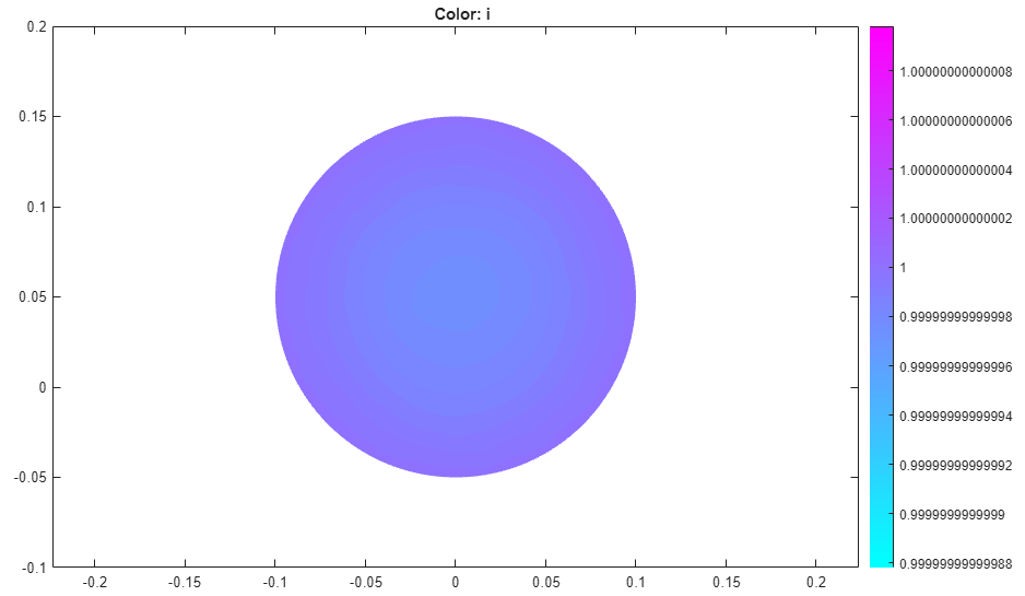
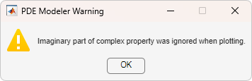
The solution of the AC power electromagnetics equation is complex. When plotting the solution, you get a warning message.
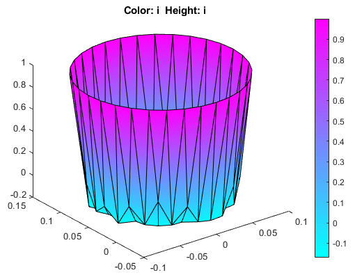
Plot the current density as a 3-D plot. To do this:
Select Plot > Parameters.
Select the Color and Height(3-D plot) options.
Select
current densityfrom the Property drop-down menu for both the Color and Height(3-D plot) options.Select Show Mesh to observe the mesh.
Due to the skin effect, the current density at the surface of the conductor is much higher than in the conductor's interior.
Improve the accuracy of the solution close to the surface by using adaptive mesh refinement. To do this:
Select Solve > Parameters.
In the resulting dialog box, select Adaptive mode.
Set the maximum numbers of triangles to
Inf.Set the maximum numbers of refinements to
1.Select the
Worst trianglesselection method.
Recompute the solution five times. Each time, the adaptive solver refines the area with the largest errors. The number of triangles is printed at the command line.
Plot the current density as a 3-D plot.

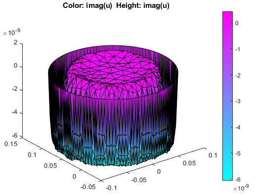
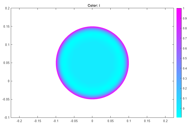
These plots show the real part of the solution, but the solution vector is the full complex solution. Plot the imaginary part of the solution. To do this:
Select Plot > Parameters.
Select the Color and Height(3-D plot) options.
Select
user entryfrom the Property drop-down menu for both Color and Height(3-D plot) options.Type
imag(u)in the corresponding User entry fields.Select Show Mesh to observe the mesh.
Observe that the skin effect depends on the frequency of the alternating current. When you increase or decrease the frequency, the skin "depth" increases or decreases, respectively. At high frequencies, only a thin layer on the surface of the wire conducts the current. At very low frequencies (approaching DC conditions), almost the entire cross section area of the wire conducts the current.
Find the solution for the angular frequencies
omega =,omega = 2*pi*50, andomega = 1E-6. Plot the real parts of the solutions in 2-D.Current density for omega = 2*pi*1000

Current density for omega = 2*pi*50
Current density for omega = 1E-6