Reduced-Order Model for Thermal Behavior of Battery
Generate a reduced-order model (ROM) to enable analysis of the spatial thermal behavior of a battery cell during a fast-charging scenario. You can use the resulting ROM in the Analyze Battery Spatial Temperature Variation During Fast Charge (Simscape Battery) example to analyze the maximum temperature gradient.

This example first sets up a 3-D thermal analysis model for a Valance:U27_36XP battery in terms of geometry, material properties, boundary conditions, and initial conditions. Partial Differential Equation Toolbox™ uses the finite element method (FEM) to discretize the model. FEM models tend to be very large, typically a few thousand to a million degrees of freedom (DoFs). Such large models are not ideal for integration into system-level modeling environments. You can reduce the finite-element model to a ROM, a much smaller system with tens to hundreds DoFs. This example uses eigenvalue decomposition or modal analysis to create a ROM. The example also adds other data required for Simscape™ analysis.
Battery Geometry
Specify the battery cell dimensions in mm.
cell_width_mm = 306;
cell_thickness_mm = 172;
cell_height_mm = 225;
cellCasing_thickness_mm = 5;
cellTab_height_mm = 8;
cellTab_radius_mm = 9;
The battery model has four main prismatic subdomains of different materials: an outer casing, a jelly roll, and positive and negative cell tabs.
First, create a cube to represent the casing.
gmCasing = fegeometry(multicuboid(cell_width_mm, cell_thickness_mm, cell_height_mm));
Next, create a jelly roll geometry. For this, create a cube representing the jelly roll by using the following calculations for the jelly roll dimension.
jellyRoll_dims = [cell_width_mm cell_thickness_mm cell_height_mm] - 2*cellCasing_thickness_mm;
gmJelly = multicuboid(jellyRoll_dims(1),jellyRoll_dims(2),jellyRoll_dims(3));
gmJelly = fegeometry(gmJelly);
Move the jelly roll geometry so that it is centered inside the casing.
gmJelly = translate(gmJelly,[0 0 cellCasing_thickness_mm]);
Now, create the tabs. For the tab geometry, create a cylinder.
tab = fegeometry(multicylinder(cellTab_radius_mm,cellTab_height_mm));
Find the required location the positive tab along the x-axis. The location of the negative tab along the x-axis is symmetrical about the origin.
jellyRoll_width_mm = jellyRoll_dims(1);
xLocTab = jellyRoll_width_mm/2 - 2*(cellTab_radius_mm + cellCasing_thickness_mm);
The tabs are centered along the y-axis.
yLocTab = 0;
The bottom of each tab sits on the top of the jelly roll.
zLocTab = cell_height_mm-cellCasing_thickness_mm;
Create two tabs by moving the tab cylinder to the required locations.
gmTab1 = translate(tab,[-xLocTab,yLocTab,zLocTab]);
gmTab2 = translate(tab,[ xLocTab,yLocTab,zLocTab]);
Combine the geometries representing the casing, jelly roll, and tabs by using the Boolean union operation.
gmCell = union(gmJelly,gmCasing,KeepBoundaries=true);
gmCell = union(gmCell,gmTab1,KeepBoundaries=true);
gmCell = union(gmCell,gmTab2,KeepBoundaries=true);
During the union operation each tab geometry gets split into two cells. Restore the tabs by merging these cells.
posTabCells = findCell(gmCell,[-xLocTab,0,cell_height_mm-cellCasing_thickness_mm/2;...
                               -xLocTab,0,cell_height_mm+cellCasing_thickness_mm/2]);

negTabCells = findCell(gmCell,[+xLocTab,0,cell_height_mm-cellCasing_thickness_mm/2;...
                               +xLocTab,0,cell_height_mm+cellCasing_thickness_mm/2]);

gmCell = mergeCells(gmCell,posTabCells);
gmCell = mergeCells(gmCell,negTabCells);
Create a string vector with identifiers for each subdomain of the battery cell.
cellDomains = ["Jelly","PositiveTab","NegativeTab","Casing"];
Find the IDs of the geometric cells corresponding to each subdomain of the battery cell.
IDX.PositiveTab = findCell(gmCell,[-xLocTab,0,cell_height_mm]);
IDX.NegativeTab = findCell(gmCell,[ xLocTab,0,cell_height_mm]);
IDX.Jelly = findCell(gmCell,[0,0,cell_height_mm/2]);
IDX.Casing = findCell(gmCell,[0,0,cellCasing_thickness_mm/2]);
Find the ID of the face at the bottom of the casing where you apply the cooling load.
IDX.cooledFaceID=nearestFace(gmCell,[0 0 -cellCasing_thickness_mm]);
Because this example uses SI units, scale the geometry to meters.
gmCell = scale(gmCell,1/1000);
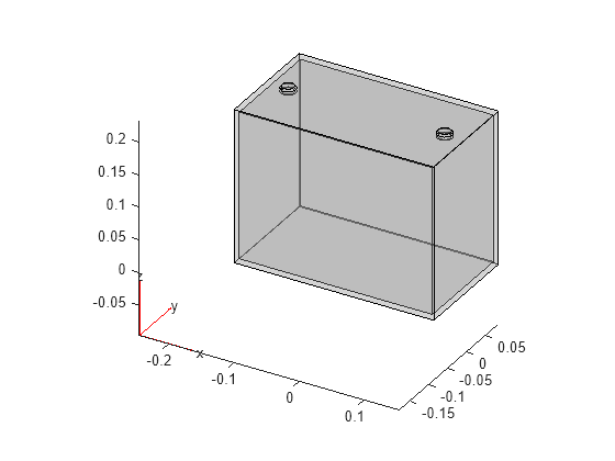
Plot the geometry.
pdegplot(gmCell,FaceAlpha=0.3)
Thermal Modal Analysis Model
Create an femodel object for modal thermal analysis and include the geometry into the model.
model = femodel(AnalysisType="thermalModal", ...
                Geometry=gmCell);
Specify the thermal conductivity, specific heat, and mass density for each subdomain. The jelly roll has an orthotropic thermal conductivity, with a large in-plane conductivity of 80 W/(K*m) and a small through-plane conductivity of 2 W/(K*m).
Define the thermal conductivity of the battery components, in W/(K*m).
cellThermalCond.inPlane = 80;
cellThermalCond.throughPlane = 2;
tabThermalCond = 386;
casingThermalCond = 50;

thermalConductivity.Jelly = [cellThermalCond.throughPlane
                             cellThermalCond.inPlane
                             cellThermalCond.inPlane];
thermalConductivity.PositiveTab = tabThermalCond;
thermalConductivity.NegativeTab = tabThermalCond;
thermalConductivity.Casing = casingThermalCond;
Define the specific heat of the battery components, in J/(kg*K).
spHeat.Jelly = 785;
spHeat.PositiveTab = 890;
spHeat.NegativeTab = 385;
spHeat.Casing = 840;
Define the mass density of the battery components, in kg/m³.
density.Jelly = 780;
density.PositiveTab = 2700;
density.NegativeTab = 8830;
density.Casing = 540;
Assign material properties to the model.
for domain = cellDomains
model.MaterialProperties(IDX.(domain)) = ...
    materialProperties(ThermalConductivity=[thermalConductivity.(domain)], ...
                       SpecificHeat=spHeat.(domain), ...
                       MassDensity=density.(domain));
end
Reduced-Order Model
Solve the modal analysis problem, and use the modal results to reduce the model for thermal analysis.
Specify the initial temperature of the battery.
T0 = 300;
model.CellIC = cellIC(Temperature=T0);
Generate the mesh.
model = generateMesh(model,Hface={model.Geometry.cellFaces(IDX.Jelly),0.03});Solve for modes of the thermal problem in a specified decay range.
Rm = solve(model,DecayRange=[-Inf,0.05]);
Use the modal results to obtain a ROM.
rom = reduce(model,ModalResults=Rm)
rom =
  ReducedThermalModel with properties:

                    K: [15×15 double]
                    M: [15×15 double]
                    F: [15×1 double]
    InitialConditions: [15×1 double]
                 Mesh: [1×1 FEMesh]
           ModeShapes: [20029×15 double]
The output rom contains a smaller-sized system to use in Simscape system-level modeling. In addition to ROM, defining a control loop requires additional data to couple the ROM with Simscape elements. The following sections create all the relevant data and populate a pde_rom structure array with it.
Unit Vectors to Load ROM in Simscape Loop
The generated ROM does not include a load or boundary conditions. The Simscape Battery™ loop computes the heat generation loads and boundary loss. To apply these loads and losses on the ROM, use unit load vectors and scale them by using scaling factors calculated from the Simscape Battery libraries. These full-length scaled load vectors with a size equal to the finite-element model DoFs are projected to reduce loads to ROM space by using the transformation matrix available in the ROM. The reduced load vectors drive the ROM dynamics.
All battery boundaries are adiabatic, except for the bottom surface where a cooling load is applied using a thermal resistance. To generate independent load vectors for all controlled loads, apply a unit loading for each controlled load and then extract the corresponding load vector. The negative sign indicates the flux directed out of the battery system.
model.FaceLoad(IDX.("cooledFaceID")) = faceLoad(Heat=-1);Assemble the finite boundary load vector corresponding to the cooled face by using assembleFEMatrices.
mats = assembleFEMatrices(model,"G");
boundaryLoad_full = full(mats.G);
Assemble load vectors corresponding to heat generation by using the sscv_unitHeatLoadBatteryROM helper function. The helper function uses assembleFEMatrices to get the source load vector.
heatGenUnit_full = ...
    sscv_unitHeatLoadBatteryROM(model,IDX.("Jelly"));
heatGenUnitPosTab_full = ...
    sscv_unitHeatLoadBatteryROM(model,IDX.("PositiveTab"));
heatGenUnitNegTab_full = ...
    sscv_unitHeatLoadBatteryROM(model,IDX.("NegativeTab"));
Thermocouple Locations to Probe Control Temperature
In the Simscape model used in Analyze Battery Spatial Temperature Variation During Fast Charge (Simscape Battery), control logic is based on temperature probed at a few spatial locations. These spatial locations are representative of typical locations of thermocouples in a physical setup. All the thermocouple locations are defined on the top surface, with tabs, of the battery. You can choose the temperature from one thermocouple, a subset of thermocouples, or the average temperature across the battery to define the control.
For simplicity, assume that each thermocouple location coincides with a mesh node, and therefore, you can use node IDs to index into the temperature vector of the solution. Identify node IDs using the coordinates of a thermocouple location.
Compute the spatial coordinates of three equally spaced thermocouples. First, compute the geometric bounding box and compute its mean.
boundingBox = [min(model.Geometry.Vertices);
               max(model.Geometry.Vertices)];
boundingBox_mean = mean(boundingBox);
Place thermocouple locations along the x-direction.
xLocations = linspace(boundingBox(1,1),boundingBox(2,1),5);
thermocouples.probe_locations = xLocations(2:end-1);
thermocouples.probe_locations(2,:) = boundingBox_mean(2);
thermocouples.probe_locations(3,:) = boundingBox_mean(3);
Find the nearest finite element mesh node for each of the thermocouple locations.
thermocouples.probeNodeIDs = ...
    model.Geometry.Mesh.findNodes(nearest=thermocouples.probe_locations);
thermocouples.numOfTempProbes = ...
    numel(thermocouples.probeNodeIDs);
The ROM solution is defined in terms of reduced DoFs. For plotting purposes, add a submatrix W of rom.TransformationMatrix that generates the temperature-time history for the nodes corresponding to thermocouple locations.
thermocouples.W = ...
    rom.TransformationMatrix(thermocouples.probeNodeIDs,:);
Lumped Thermal Mass of Cell
Define the cell thermal mass required in the Battery (Table-Based) library component.
cellThermalMass = 0;
for domain = cellDomains
    volume.(domain) = ...
        model.Geometry.Mesh.volume(model.Geometry.Mesh.findElements("region", ...
                                                       Cell=IDX.(domain)));
    cellThermalMass = ...
        cellThermalMass + ...
        volume.(domain).*density.(domain).*spHeat.(domain);
end
Array with Data Required for Simscape Model
Add all the remaining required data to the pde_rom structure array.
Add the initial temperature of the battery, in K.
pde_rom.prop.initialTemperature = T0;
Add the weld resistance value of the battery cell tabs, in ohm.
pde_rom.prop.cellTab_weldR = 7.5e-4;
Add the bottom cooling area.
pde_rom.prop.coolingArea_sqm = cell_width_mm* ...
                               cell_thickness_mm*1e-6;
Add the cell geometry data.
pde_rom.prop.cell_width_mm = cell_width_mm;
pde_rom.prop.cell_thickness_mm = cell_thickness_mm;
pde_rom.prop.cell_height_mm = cell_height_mm;
pde_rom.prop.cellCasing_thickness_mm = cellCasing_thickness_mm;
pde_rom.prop.cellTab_height_mm = cellTab_height_mm;
pde_rom.prop.cellTab_radius_mm = cellTab_radius_mm;
pde_rom.Geometry = model.Geometry;
pde_rom.prop.volume = volume;
Add the cell material data.
pde_rom.prop.cellThermalCond.inPlane = cellThermalCond.inPlane;
pde_rom.prop.cellThermalCond.throughPlane = ...
                                  cellThermalCond.throughPlane;
pde_rom.prop.tabThermalCond = tabThermalCond;
pde_rom.prop.casingThermalCond = casingThermalCond;
pde_rom.prop.thermalConductivity = thermalConductivity;
pde_rom.prop.density = density;
pde_rom.prop.spHeat = spHeat;
pde_rom.prop.cellThermalMass = cellThermalMass;
Add the thermal load vectors.
pde_rom.Q.boundaryLoad_full = boundaryLoad_full;
pde_rom.Q.heatGenUnit_full = heatGenUnit_full;
pde_rom.Q.heatGenUnitPosTab_full = heatGenUnitPosTab_full;
pde_rom.Q.heatGenUnitNegTab_full = heatGenUnitNegTab_full;
Add the thermocouples data.
pde_rom.thermocouples = thermocouples;
Add the thermal ROM.
pde_rom.rom = rom
pde_rom = struct with fields:
             prop: [1×1 struct]
         Geometry: [1×1 fegeometry]
                Q: [1×1 struct]
    thermocouples: [1×1 struct]
              rom: [1×1 pde.ReducedThermalModel]
Save the struct array to a MAT-file. You can use the resulting MAT-file in Simscape Battery to analyze the battery temperature gradient during fast charging. Using the MAT-file does not require Partial Differential Equation Toolbox.
save sscv_BatteryCellSpatialTempVariation_rom pde_rom
clearvars -except pde_rom