Output Function for Problem-Based Optimization
This example shows how to use an output function to plot and store the history of the iterations for a nonlinear problem. This history includes the evaluated points, the search directions that the solver uses to generate points, and the objective function values at the evaluated points.
For the solver-based approach to this example, see Output Functions for Optimization Toolbox.
Plot functions have the same syntax as output functions, so this example also applies to plot functions.
For both the solver-based approach and the problem-based approach, write the output function according to the solver-based approach. In the solver-based approach, you use a single vector variable, usually denoted x, instead of a collection of optimization variables of various sizes. So to write an output function for the problem-based approach, you must understand the correspondence between your optimization variables and the single solver-based x. To map between optimization variables and x, use varindex. In this example, to avoid confusion with an optimization variable named x, use "in" as the vector variable name.
Problem Description
The problem is to minimize the following function of variables x and y:
In addition, the problem has two nonlinear constraints:
Problem-Based Setup
To set up the problem in the problem-based approach, define optimization variables and an optimization problem object.
x = optimvar("x");
y = optimvar("y");
prob = optimproblem;
Define the objective function as an expression in the optimization variables.
f = exp(x)*(4*x^2 + 2*y^2 + 4*x*y + 2*y + 1);
Include the objective function in prob.
prob.Objective = f;
To include the nonlinear constraints, create optimization constraint expressions.
cons1 = x + y - x*y >= 1.5;
cons2 = x*y >= -10;
prob.Constraints.cons1 = cons1;
prob.Constraints.cons2 = cons2;
Because this is a nonlinear problem, you must include an initial point structure x0. Use x0.x = –1 and x0.y = 1.
x0.x = -1;
x0.y = 1;
Output Function
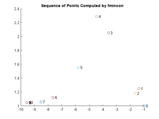
The outfun output function records a history of the points generated by fmincon during its iterations. The output function also plots the points and keeps a separate history of the search directions for the sqp algorithm. The search direction is a vector from the previous point to the next point that fmincon tries. During its final step, the output function saves the history in workspace variables, and saves a history of the objective function values at each iterative step.
For the required syntax of optimization output functions, see Output Function and Plot Function Syntax.
An output function takes a single vector variable as an input. But the current problem has two variables. To find the mapping between the optimization variables and the input variable, use varindex.
idx = varindex(prob);
idx.x
ans =
1
idx.y
ans =
2
The mapping shows that x is variable 1 and y is variable 2. So, if the input variable is named in, then x = in(1) and y = in(2).
function stop = outfun(in,optimValues,state,idx)
     persistent history searchdir fhistory
     stop = false;

     switch state
         case "init"
             hold on
             history = [];
             fhistory = [];
             searchdir = [];
         case "iter"
         % Concatenate current point and objective function
         % value with history. in must be a row vector.
           fhistory = [fhistory; optimValues.fval];
           history = [history; in(:)']; % Ensure in is a row vector
         % Concatenate current search direction with
         % searchdir.
           searchdir = [searchdir;...
                        optimValues.searchdirection(:)'];
           plot(in(idx.x),in(idx.y),"o");
         % Label points with iteration number and add title.
         % Add .15 to idx.x to separate label from plotted "o"
           text(in(idx.x)+.15,in(idx.y),...
                num2str(optimValues.iteration));
           title("Sequence of Points Computed by fmincon");
         case "done"
             hold off
             assignin("base",optimhistory=history);
             assignin("base",searchdirhistory=searchdir);
             assignin("base",functionhistory=fhistory);
         otherwise
     end
 end
Include the output function in the optimization by setting the OutputFcn option. Also, set the Algorithm option to use the "sqp" algorithm instead of the default "interior-point" algorithm. Pass idx to the output function as an extra parameter in the last input. See Passing Extra Parameters.
outputfn = @(in,optimValues,state)outfun(in,optimValues,state,idx);
opts = optimoptions("fmincon",Algorithm="sqp",OutputFcn=outputfn);
Run Optimization Using Output Function
Run the optimization, including the output function, by using the "Options" name-value pair argument.
[sol,fval,eflag,output] = solve(prob,x0,Options=opts)
Solving problem using fmincon.
Local minimum found that satisfies the constraints.

Optimization completed because the objective function is non-decreasing in
feasible directions, to within the value of the optimality tolerance,
and constraints are satisfied to within the value of the constraint tolerance.

<stopping criteria details>
sol = struct with fields:
    x: -9.5474
    y: 1.0474
fval =
0.0236
eflag =
    OptimalSolution
output = struct with fields:
              iterations: 10
               funcCount: 22
               algorithm: 'sqp'
                 message: 'Local minimum found that satisfies the constraints.↵↵Optimization completed because the objective function is non-decreasing in ↵feasible directions, to within the value of the optimality tolerance,↵and constraints are satisfied to within the value of the constraint tolerance.↵↵<stopping criteria details>↵↵Optimization completed: The relative first-order optimality measure, 7.127069e-10,↵is less than options.OptimalityTolerance = 1.000000e-06, and the relative maximum constraint↵violation, 1.065814e-14, is less than options.ConstraintTolerance = 1.000000e-06.'
         constrviolation: 1.0658e-14
                stepsize: 1.4893e-07
            lssteplength: 1
           firstorderopt: 7.1271e-10
            bestfeasible: [1×1 struct]
     objectivederivative: 'reverse-AD'
    constraintderivative: 'closed-form'
                  solver: 'fmincon'
Examine the iteration history. Each row of the optimhistory matrix represents one point. The last few points are very close, which explains why the plotted sequence shows overprinted numbers for points 8, 9, and 10.
disp("Locations");disp(optimhistory)Locations -1.0000 1.0000 -1.3679 1.2500 -1.6509 1.1813 -3.5870 2.0537 -4.4574 2.2895 -5.8015 1.5531 -7.6498 1.1225 -8.5223 1.0572 -9.5463 1.0464 -9.5474 1.0474 -9.5474 1.0474
Examine the searchdirhistory and functionhistory arrays.
disp("Search Directions");disp(searchdirhistory)Search Directions
0 0
-0.3679 0.2500
-0.2831 -0.0687
-1.9360 0.8725
-0.8704 0.2358
-1.3441 -0.7364
-2.0877 -0.6493
-0.8725 -0.0653
-1.0240 -0.0108
-0.0011 0.0010
0.0000 -0.0000
disp("Function Values");disp(functionhistory)Function Values
1.8394
1.8513
1.7757
0.9839
0.6343
0.3250
0.0978
0.0517
0.0236
0.0236
0.0236
Unsupported Functions Require fcn2optimexpr
If your objective function or nonlinear constraint functions are not composed of elementary functions, you must convert the functions to optimization expressions using fcn2optimexpr. See Convert Nonlinear Function to Optimization Expression. For this example, you would enter the following code:
fun = @(x,y)exp(x)*(4*x^2 + 2*y^2 + 4*x*y + 2*y + 1);
f = fcn2optimexpr(fun,x,y);
For the list of supported functions, see Supported Operations for Optimization Variables and Expressions.