Optimal Dispatch of Power Generators: Solver-Based
This example shows how to schedule two gas-fired electric generators optimally, meaning to get the most revenue minus cost. While the example is not entirely realistic, it does show how to take into account costs that depend on decision timing.
For the problem-based approach to this problem, see Optimal Dispatch of Power Generators: Problem-Based.
Problem Definition
The electricity market has different prices at different times of day. If you have generators, you can take advantage of this variable pricing by scheduling your generators to operate when prices are high. Suppose that there are two generators that you control. Each generator has three power levels (off, low, and high). Each generator has a specified rate of fuel consumption and power production at each power level. Of course, fuel consumption is 0 when the generator is off.
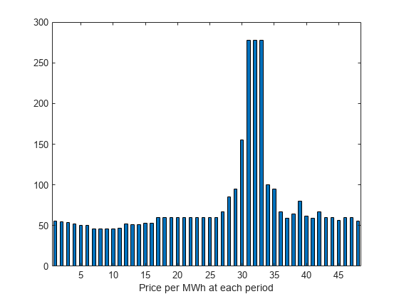
You can assign a power level to each generator during each half-hour time interval during a day (24 hours, so 48 intervals). Based on historical records, you can assume that you know the revenue per megawatt-hour (MWh) that you get in each time interval. The data for this example is from the Australian Energy Market Operator https://www.nemweb.com.au/REPORTS/CURRENT/ in mid-2013, and is used under their terms https://www.aemo.com.au/privacy-and-legal-notices/copyright-permissions.
load dispatchPrice; % Get poolPrice, which is the revenue per MWh
bar(poolPrice,.5)
xlim([.5,48.5])
xlabel("Price per MWh at each period")
There is a cost to start a generator after it has been off. The other constraint is a maximum fuel usage for the day. The maximum fuel constraint is because you buy your fuel a day ahead of time, so can use only what you just bought.
Problem Notation and Parameters
You can formulate the scheduling problem as a binary integer programming problem as follows. Define indexes i, j, and k, and a binary scheduling vector y as:
nPeriods= the number of time periods, 48 in this case.i= a time period, 1 <=i<= 48.j= a generator index, 1 <=j<= 2 for this example.y(i,j,k) = 1when periodi, generatorjis operating at power levelk. Let low power bek = 1, and high power bek = 2. The generator is off whensum_k y(i,j,k) = 0.
You need to determine when a generator starts after being off. Let
z(i,j) = 1when generatorjis off at periodi, but is on at periodi + 1.z(i,j) = 0otherwise. In other words,z(i,j) = 1whensum_k y(i,j,k) = 0andsum_k y(i+1,j,k) = 1.
Obviously, you need a way to set z automatically based on the settings of y. A linear constraint below handles this setting.
You also need the parameters of the problem for costs, generation levels for each generator, consumption levels of the generators, and fuel available.
poolPrice(i)-- Revenue in dollars per MWh in intervali.gen(j,k)-- MW generated by generatorjat power levelk.fuel(j,k)-- Fuel used by generatorjat power levelk.totalfuel-- Fuel available in one day.startCost-- Cost in dollars to start a generator after it has been off.fuelPrice-- Cost for a unit of fuel.
You got poolPrice when you executed load dispatchPrice;. Set the other parameters as follows.
fuelPrice = 3;
totalfuel = 3.95e4;
nPeriods = length(poolPrice); % 48 periods
nGens = 2; % Two generators
gen = [61,152;50,150]; % Generator 1 low = 61 MW, high = 152 MW
fuel = [427,806;325,765]; % Fuel consumption for generator 2 is low = 325, high = 765
startCost = 1e4; % Cost to start a generator after it has been off
Generator Efficiency
Examine the efficiency of the two generators at their two operating points.
efficiency = gen./fuel; % Calculate electricity per unit fuel use
rr = efficiency'; % for plotting
h = bar(rr);
h(1).FaceColor = "g";
h(2).FaceColor = "c";
legend(h,"Generator 1","Generator 2",Location="northeastoutside")
ax = gca;
ax.XTick = [1,2];
ax.XTickLabel = {"Low","High"};
ylim([.1,.2])
ylabel("Efficiency")
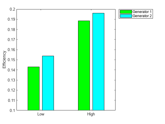
Notice that generator 2 is a bit more efficient than generator 1 at its corresponding operating points (low or high), but generator 1 at its high operating point is more efficient than generator 2 at its low operating point.
Variables for Solution
To set up the problem, you need to encode all the problem data and constraints in the form that the intlinprog solver requires. You have variables y(i,j,k) that represent the solution of the problem, and z(i,j) auxiliary variables for charging to turn on a generator. y is an nPeriods-by-nGens-by-2 array, and z is an nPeriods-by-nGens array.
To put these variables in one long vector, define the variable of unknowns x:
x = [y(:);z(:)];
For bounds and linear constraints, it is easiest to use the natural array formulation of y and z, then convert the constraints to the total decision variable, the vector x.
Bounds
The solution vector x consists of binary variables. Set up the bounds lb and ub.
lby = zeros(nPeriods,nGens,2); % 0 for the y variables
lbz = zeros(nPeriods,nGens); % 0 for the z variables
lb = [lby(:);lbz(:)]; % Column vector lower bound
ub = ones(size(lb)); % Binary variables have lower bound 0, upper bound 1
Linear Constraints
For linear constraints A*x <= b, the number of columns in the A matrix must be the same as the length of x, which is the same as the length of lb. To create rows of A of the appropriate size, create zero matrices of the sizes of the y and z matrices.
cleary = zeros(nPeriods,nGens,2);
clearz = zeros(nPeriods,nGens);
To ensure that the power level has no more than one component equal to 1, set a linear inequality constraint:
x(i,j,1) + x(i,j,2) <= 1
A = spalloc(nPeriods*nGens,length(lb),2*nPeriods*nGens); % nPeriods*nGens inequalities
counter = 1;
for ii = 1:nPeriods
    for jj = 1:nGens
        temp = cleary;
        temp(ii,jj,:) = 1;
        addrow = [temp(:);clearz(:)]';
        A(counter,:) = sparse(addrow);
        counter = counter + 1;
    end
end
b = ones(nPeriods*nGens,1); % A*x <= b means no more than one of x(i,j,1) and x(i,j,2) are equal to 1
The running cost per period is the cost for fuel for that period. For generator j operating at level k, the cost is fuelPrice * fuel(j,k).
To ensure that the generators do not use too much fuel, create an inequality constraint on the sum of fuel usage.
yFuel = lby; % Initialize fuel usage array
yFuel(:,1,1) = fuel(1,1); % Fuel use of generator 1 in low setting
yFuel(:,1,2) = fuel(1,2); % Fuel use of generator 1 in high setting
yFuel(:,2,1) = fuel(2,1); % Fuel use of generator 2 in low setting
yFuel(:,2,2) = fuel(2,2); % Fuel use of generator 2 in high setting

addrow = [yFuel(:);clearz(:)]';
A = [A;sparse(addrow)];
b = [b;totalfuel]; % A*x <= b means the total fuel usage is <= totalfuel
Set the Generator Startup Indicator Variables
How can you get the solver to set the z variables automatically to match the active/off periods that the y variables represent? Recall that the condition to satisfy is z(i,j) = 1 exactly when
sum_k y(i,j,k) = 0 and sum_k y(i+1,j,k) = 1.
Notice that
sum_k ( - y(i,j,k) + y(i+1,j,k) ) > 0 exactly when you want z(i,j) = 1.
Therefore, include the linear inequality constraints
sum_k ( - y(i,j,k) + y(i+1,j,k) ) - z(i,j) < = 0
in the problem formulation, and include the z variables in the objective function cost. By including the z variables in the objective function, the solver attempts to lower the values of the z variables, meaning it tries to set them all equal to 0. But for those intervals when a generator turns on, the linear inequality forces the z(i,j) to equal 1.
Add extra rows to the linear inequality constraint matrix A to represent these new inequalities. Wrap around the time so that interval 1 logically follows interval 48.
tempA = spalloc(nPeriods*nGens,length(lb),2*nPeriods*nGens);
counter = 1;
for ii = 1:nPeriods
    for jj = 1:nGens
        temp = cleary;
        tempy = clearz;
        temp(ii,jj,1) = -1;
        temp(ii,jj,2) = -1;
        if ii < nPeriods % Intervals 1 to 47
            temp(ii+1,jj,1) = 1;
            temp(ii+1,jj,2) = 1;
        else % Interval 1 follows interval 48
            temp(1,jj,1) = 1;
            temp(1,jj,2) = 1;
        end
        tempy(ii,jj) = -1;
        temp = [temp(:);tempy(:)]'; % Row vector for inclusion in tempA matrix
        tempA(counter,:) = sparse(temp);
        counter = counter + 1;
    end
end
A = [A;tempA];
b = [b;zeros(nPeriods*nGens,1)]; % A*x <= b sets z(i,j) = 1 at generator startup
Sparsity of Constraints
If you have a large problem, using sparse constraint matrices saves memory, and can save computational time as well. The constraint matrix A is quite sparse:
filledfraction = nnz(A)/numel(A)
filledfraction =
0.0155
intlinprog accepts sparse linear constraint matrices A and Aeq, but requires their corresponding vector constraints b and beq to be full.
Define Objective
The objective function includes fuel costs for running the generators, revenue from running the generators, and costs for starting the generators.
generatorlevel = lby; % Generation in MW, start with 0s
generatorlevel(:,1,1) = gen(1,1); % Fill in the levels
generatorlevel(:,1,2) = gen(1,2);
generatorlevel(:,2,1) = gen(2,1);
generatorlevel(:,2,2) = gen(2,2);
Incoming revenue = x.*generatorlevel.*poolPrice
revenue = generatorlevel; % Allocate revenue array
for ii = 1:nPeriods
    revenue(ii,:,:) = poolPrice(ii)*generatorlevel(ii,:,:);
end
Total fuel cost = y.*yFuel*fuelPrice
fuelCost = yFuel*fuelPrice;
Startup cost = z.*ones(size(z))*startCost
starts = (clearz + 1)*startCost;
starts = starts(:); % Generator startup cost vector
The vector x = [y(:);z(:)]. Write the total profit in terms of x:
profit = Incoming revenue - Total fuel cost - Startup cost
f = [revenue(:) - fuelCost(:);-starts]; % f is the objective function vectorSolve the Problem
To save space, suppress iterative display.
options = optimoptions("intlinprog",Display="final");
[x,fval,eflag,output] = intlinprog(-f,1:length(f),A,b,[],[],lb,ub,options);
Optimal solution found.

Intlinprog stopped because the objective value is within a gap tolerance of the optimal value, options.RelativeGapTolerance = 0.0001. The intcon variables are integer within tolerance, options.ConstraintTolerance = 1e-06.
Examine the Solution
The easiest way to examine the solution is dividing the solution vector x into its two components, y and z.
ysolution = x(1:nPeriods*nGens*2);
zsolution = x(nPeriods*nGens*2+1:end);
ysolution = reshape(ysolution,[nPeriods,nGens,2]);
zsolution = reshape(zsolution,[nPeriods,nGens]);
Plot the solution as a function of time.
subplot(3,1,1)
bar(ysolution(:,1,1)*gen(1,1)+ysolution(:,1,2)*gen(1,2),.5,"g")
xlim([.5,48.5])
ylabel("MWh")
title("Generator 1 optimal schedule",FontWeight="bold")
subplot(3,1,2)
bar(ysolution(:,2,1)*gen(2,1)+ysolution(:,2,2)*gen(2,2),.5,"c")
title("Generator 2 optimal schedule",FontWeight="bold")
xlim([.5,48.5])
ylabel("MWh")
subplot(3,1,3)
bar(poolPrice,.5)
xlim([.5,48.5])
title("Energy price",FontWeight="bold")
xlabel("Period")
ylabel("$ / MWh")
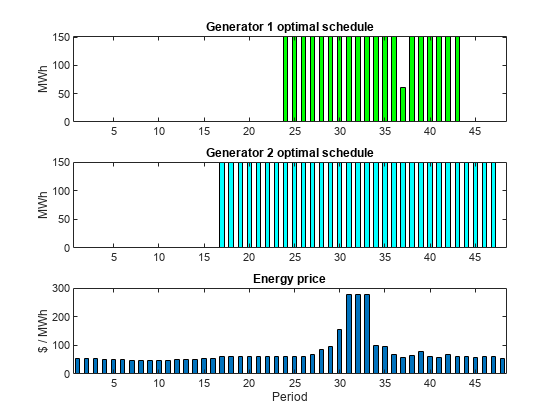
Generator 2 runs longer than generator 1, which you would expect because it is more efficient. Generator 2 runs at its high power level whenever it is on. Generator 1 runs mainly at its high power level, but dips down to low power for one time unit. Each generator runs for one contiguous set of periods daily, so incurs only one startup cost.
Check that the z variable is 1 for the periods when the generators start.
starttimes = find(round(zsolution) == 1); % Use round for noninteger results
[theperiod,thegenerator] = ind2sub(size(zsolution),starttimes)
theperiod = 2×1
23
16
thegenerator = 2×1

     1
     2
The periods when the generators start match the plots.
Compare to Lower Penalty for Startup
If you choose a small value of startCost, the solution involves multiple generation periods.
startCost = 500; % Choose a lower penalty for starting the generators
starts = (clearz + 1)*startCost;
starts = starts(:); % Start cost vector
fnew = [revenue(:) - fuelCost(:);-starts]; % New objective function
[xnew,fvalnew,eflagnew,outputnew] = ...
    intlinprog(-fnew,1:length(fnew),A,b,[],[],lb,ub,options);
Optimal solution found.

Intlinprog stopped at the root node because the objective value is within a gap tolerance of the optimal value, options.RelativeGapTolerance = 0.0001. The intcon variables are integer within tolerance, options.ConstraintTolerance = 1e-06.
ysolutionnew = xnew(1:nPeriods*nGens*2);
zsolutionnew = xnew(nPeriods*nGens*2+1:end);
ysolutionnew = reshape(ysolutionnew,[nPeriods,nGens,2]);
zsolutionnew = reshape(zsolutionnew,[nPeriods,nGens]);

subplot(3,1,1)
bar(ysolutionnew(:,1,1)*gen(1,1)+ysolutionnew(:,1,2)*gen(1,2),.5,"g")
xlim([.5,48.5])
ylabel("MWh")
title("Generator 1 optimal schedule",FontWeight="bold")
subplot(3,1,2)
bar(ysolutionnew(:,2,1)*gen(2,1)+ysolutionnew(:,2,2)*gen(2,2),.5,"c")
title("Generator 2 optimal schedule",FontWeight="bold")
xlim([.5,48.5])
ylabel("MWh")
subplot(3,1,3)
bar(poolPrice,.5)
xlim([.5,48.5])
title("Energy price",FontWeight="bold")
xlabel("Period")
ylabel("$ / MWh")
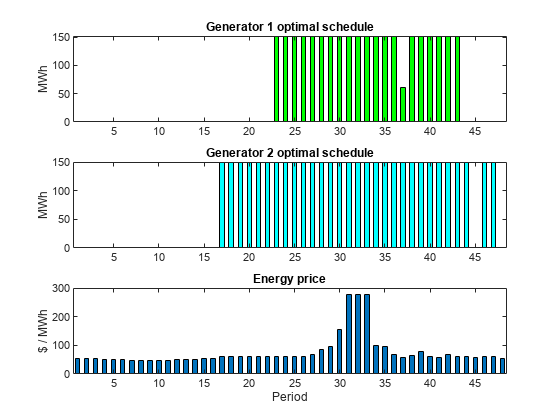
starttimes = find(round(zsolutionnew) == 1); % Use round for noninteger results
[theperiod,thegenerator] = ind2sub(size(zsolution),starttimes)
theperiod = 3×1
22
16
45
thegenerator = 3×1

     1
     2
     2