ADC Linearity Measurement Using Histogram
Statistical measurement of ADC Linearity is popular in physical systems due to its noise tolerance and relative simplicity of implementation in a physical environment. This example covers problems inherent to statistical linearity measurements and some possible solutions for implementing these measurements in Simulink®.
The Model
A histogram-based linearity measurement can be broken into five sections:
Stimulus
Device Under Test (DUT)
Preprocessing
Histogram Computation
Linearity Measurement
The problems inherent to the statistical method occur primarily in the Stimulus and Preprocessing sections. The stimulus signal needs to be uniform over the ADC's input to give a flat histogram for an unimpaired converter, while the preprocessing needs to ensure that exactly one period of the stimulus is binned by the histogram at a time.
Alternatively, the stimulus frequency can be nonuniform but the histogram must be manipulated using the PDF of the nonuniform input so as to remove the influence of the nonuniformity on the result.
s = warning('off', 'Simulink:blocks:DivideByZero');
model = 'histogramLinearityExample';
open_system(model);
set_param([model '/Flash ADC'], 'EnableLinearityImpairments', 'off');

The sawtooth stimulus frequency automatically adapts to different combinations of simulation runtime and converter number of bits.

 and
and  are defined in Range,
  is defined in the model parameter StopTime,
  is defined by Fs and
  is defined by Nbits.
  serves to prevent a frequency of 0 in the case of a non-finite simulation time. Otherwise, the sawtooth period takes the entire simulation time.
Buffering
In this model, the samples are buffered separately from the histogram computation for two reasons. First, it is important that the histogram updates at an integer multiple of the stimulus period. This ensures that the histogram has the correct shape. Second, the number of samples per period of the sawtooth stimulus is dependent on its frequency and the frequency of the conversion start signal, which is the sampling frequency. Therefore, the number of samples to buffer is the sample frequency divided by the sawtooth frequency.

The buffer block causes its own problem while ensuring histogram uniformity. The initial output of the buffer is passed to the histogram at the start of simulation, effectively a buffer full of zeros all determined by an initial condition.
model3 = 'histogramInitialCondition';
load_system(model3);
%open_system([model '/Histogram']);
out=sim(model3);
plot(out.ADCHistogram,'-rd');
grid on;
title('Histogram');
ylabel('Amplitude');
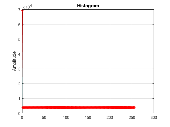
The resulting histogram is corrupted by the massive spike at 0, due to the propagation of the initial condition.
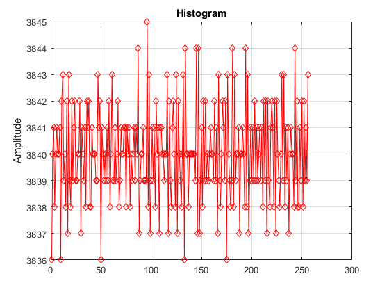
The MATLAB Function block in the Histogram section keeps the histogram disabled until the next buffer, the first one filled with simulation data, arrives at the histogram. Therefore, this prevents the final histogram from being dependent on initial conditions.
open_system(model);
set_param([model '/Flash ADC'], 'EnableLinearityImpairments', 'off');
out=sim(model);
plot(out.ADCHistogram,'-rd');
grid on;
title('Histogram');
ylabel('Amplitude');
Input Uniformity
A ramp or sawtooth input provides a linear sweep of all of the values over the ADC's dynamic range.
However, due to threshold placement in ADCs, an ideal ADC's transfer curve is not centered in its dynamic range; the ideal transfer curve is left shifted by 0.5 LSB. Therefore, the first threshold is at 0.5 LSB and the last threshold is 1.5 LSB lower than the maximum dynamic range. Compensate for this effect by adding a -0.5 LSB bias to the stimulus.
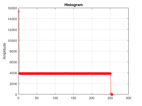
More severe problems occur with converters that have large offset and/or gain errors. Specifically, if the offset error is lower than -1 LSB or the full scale error (the sum of offset and gain error) exceeds 1 LSB, some codes at the bottom or top of the transfer curve (respectively) will be measured as missing, regardless of their actual functionality. Knowing this, statistical linearity measurement techniques should only be applied after offset and gain errors have been corrected.
set_param([model '/Flash ADC'], 'EnableLinearityImpairments', 'on');
set_param([model '/Flash ADC'], 'OffsetError', '3');
set_param([model '/Flash ADC'], 'GainError', '2');
%open_system([model '/Histogram']);
out=sim(model);
plot(out.ADCHistogram,'-rd');
grid on;
title('Histogram');
ylabel('Amplitude');
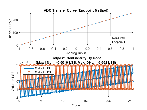
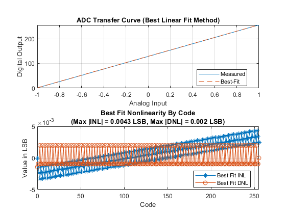
To measure the full transfer curve of an ADC with large offset and/or full scale errors in Simulink®, use the ADC DC Measurement block or the ADC Testbench. Configuration of the stimulus to cover the whole ADC transfer curve will not effect these blocks' results the way it will effect the histogram.
model2 = 'flashWithTestbench';
open_system(model2);
set_param([model2 '/Flash ADC'], 'EnableLinearityImpairments', 'off');
set_param([model2 '/Flash ADC'], 'OffsetError', '3');
set_param([model2 '/Flash ADC'], 'GainError', '2');
sim(model2);
msblks.ADC.adcDcMeasurementPlot([model2 '/ADC DC Measurement']);

Linearity Measurement
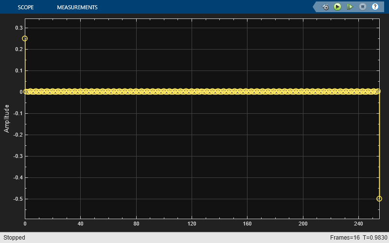
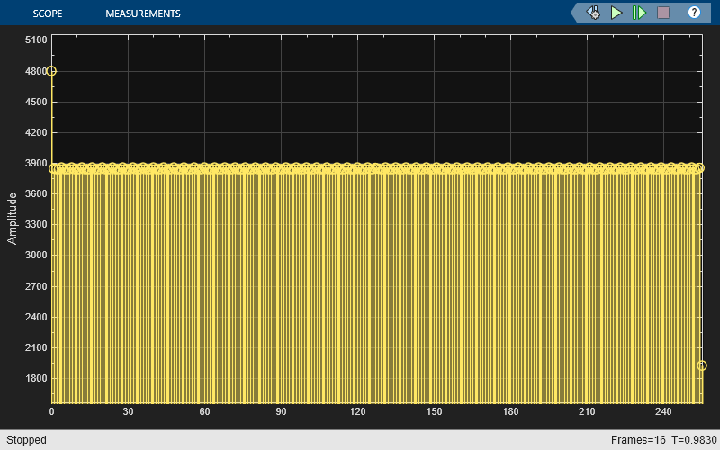
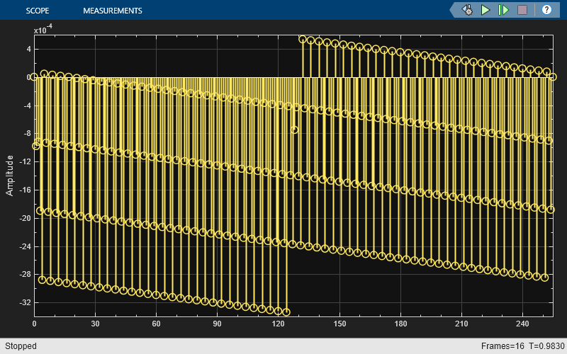
With the input and preprocessing conditions met, the histogram provides an excellent visual representation of the linearity of the data converter. A set of mathematical operations applied to this histogram yield measurements for both DNL and INL.
set_param([model '/Flash ADC'], 'EnableLinearityImpairments', 'on');
set_param([model '/Flash ADC'], 'OffsetError', '0.25');
set_param([model '/Flash ADC'], 'GainError', '0.25');

set_param([model '/Differential Nonlinearity'],'Commented','off');
set_param([model '/Integral Nonlinearity'],'Commented','off');
set_param([model '/Histogram'],'Commented','off');

open_system([model '/Differential Nonlinearity']);
open_system([model '/Integral Nonlinearity']);
open_system([model '/Histogram']);
sim(model);
open_system([model '/Hist2DNL']);
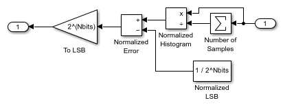
INL is subsequently computed from DNL.
open_system([model '/DNL2INL']);

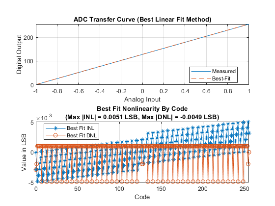
Endpoint INL computed in this manner is equivalent to the endpoint INL computed by the ADC DC Measurement block, though the ADC DC Measurement block does not report full scale DNL.
open_system(model2);
set_param([model2 '/Flash ADC'], 'EnableLinearityImpairments', 'on');
set_param([model2 '/Flash ADC'], 'OffsetError', '0.25');
set_param([model2 '/Flash ADC'], 'GainError', '0.25');
sim(model2);
msblks.ADC.adcDcMeasurementPlot([model2 '/ADC DC Measurement']);

warning(s.state, 'Simulink:blocks:DivideByZero');