Time-Varying MPC Control of an Inverted Pendulum on a Cart
This example shows how to control an inverted pendulum on a cart using a linear time-varying model predictive controller (LTV MPC).
Pendulum/Cart Assembly
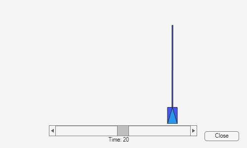
The plant for this example is the following pendulum/cart assembly, where z is the cart position and theta is the pendulum angle.

The manipulated variable for this system is a variable force F acting on the cart. The range of the force is between -100 and 100 (MKS units are assumed). The controller needs to keep the pendulum upright while moving the cart to a new position or when the pendulum is nudged forward by an impulse disturbance dF applied at the upper end of the inverted pendulum.
Control Objectives
Assume the following initial conditions for the pendulum/cart assembly:
The cart is stationary at z =
0.
The inverted pendulum is stationary at the upright position theta =
0.
The control objectives are:
Cart can be moved to a new position between
-20and20with a step setpoint change.
When tracking such a setpoint change, the rise time should be less than 4 seconds (for performance) and the overshoot should be less than
10percent (for robustness).
When an impulse disturbance of magnitude of
4is applied to the pendulum, the cart and pendulum should return to its original position with small displacement.
The upright position is an unstable equilibrium for the inverted pendulum, which makes the control task more challenging.
Choice of Time-Varying MPC
In MPC Control of an Inverted Pendulum on a Cart, a single MPC controller is able to move the cart to a new position between -10 and 10. However, if you increase the step setpoint change to 20, the pendulum fails to recover its upright position during the transition.
To reach the longer distance within the same rise time, the controller applies more force to the cart at the beginning. As a result, the pendulum is displaced from its upright position by a larger angle, such as 60 degrees. At such angles, the plant dynamics differ significantly from the LTI predictive model obtained at theta = 0. As a result, errors in the prediction of plant behavior exceed what the built-in MPC robustness can handle, and the controller fails to perform properly.
To avoid the pendulum falling, a simple workaround is to restrict pendulum displacement by adding soft output constraints to theta and reducing the ECR weight (from the default value of 1e5 to 100) to soften the constraints.
mpcobj.OV(2).Min = -pi/2;
mpcobj.OV(2).Max = pi/2;
mpcobj.Weights.ECR = 100;
However, with these new controller settings it is no longer possible to reach the longer distance within the required rise time. In other words, controller performance is sacrificed to avoid violation of the soft output constraints.
To move the cart to a new position between -20 and 20 while maintaining the same rise time, the controller needs to have more accurate models at different angles so that the controller can use them for better prediction. Adaptive MPC allows you to solve a nonlinear control problem by updating linear time-varying plant models at run time.
Control Structure
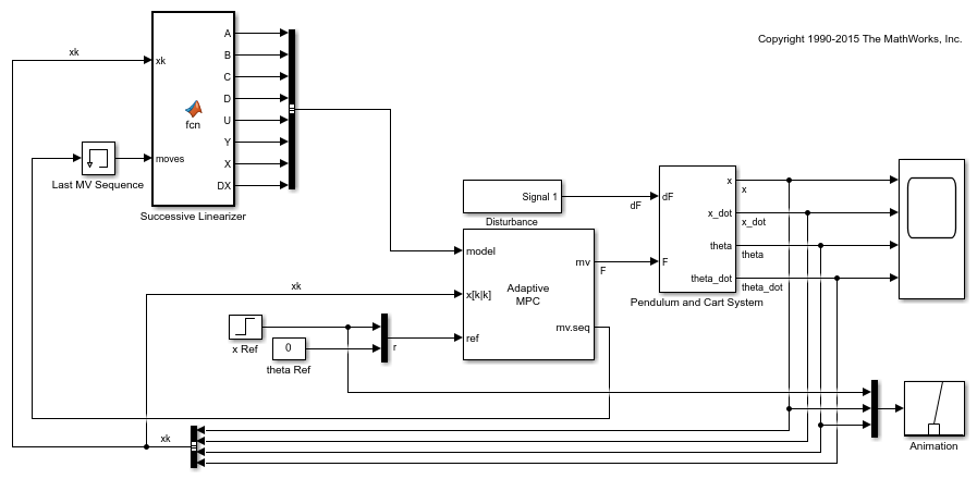
For this example, use a single LTV MPC controller with:
One manipulated variable: Variable force F.
Two measured outputs: Cart position z and pendulum angle theta.
mdlMPC = 'mpc_pendcartLTVMPC';
open_system(mdlMPC);

Because all the plant states are measurable, they are directly used as custom estimated states in the Adaptive MPC block.
While the cart position setpoint varies (step input), the pendulum angle setpoint is constant (0 = upright position).
Linear Time-Varying Plant Models
At each control interval, LTV MPC requires a linear plant model for each prediction step, from current time k to time k+p, where p is the prediction horizon.
The system is described by the following equations, where l is the distance to the pendulum center of mass, m and M are the masses of the pendulum and the cart, respectively, and Kd is a viscous friction damping term.


From the second equation, you can derive a formula expressing the angular acceleration as a function of the angular and linear velocities by collecting the length l in the second term, the cosine of theta in the last term, and isolating the second derivative of theta on the left hand side. For a thorough explanation of how the equations are derived, see Derive Equations of Motion and Simulate Cart-Pole System (Symbolic Math Toolbox).
In this example, the equations are defined in the pendulumCT function. For more details, see the pendulumCT.m file. For a thorough explanation of how the equations are derived, see
The Successive Linearizer block in the Simulink® model generates the LTV models at run time. At each prediction step, the block obtains state-space matrices A, B, C, and D using a Jacobian in continuous-time, and then converts them into discrete-time values. The initial plant states x(k) are directly measured from the plant. The plant input sequence contains the optimal moves generated by the MPC controller in the previous control interval.
Simulink Plant
The system equations can be rewritten as follows (for details see Derive Equations of Motion and Simulate Cart-Pole System (Symbolic Math Toolbox)).


From the second equation, you can derive a formula expressing the angular acceleration as a function of the angular and linear velocities by collecting the length l in the second term, the cosine of theta in the last term, and isolating the second derivative of theta on the left hand side.
The plant uses these equations, implemented in Simulink using basic blocks, in the Pendulum and Cart System subsystem.
open_system([mdlMPC '/Pendulum and Cart System'],'force')

Adaptive MPC Design
The MPC controller is designed at its nominal equilibrium operating point.
x0 = zeros(4,1);
u0 = zeros(1,1);
Analytically obtain a linear plant model using the ODEs.
[~,~,A,B,C,D] = pendulumCT(x0, u0);
plant = ss(A,B,C([1 3],:),D([1 3],:)); % position and angle
To control an unstable plant, the controller sample time cannot be too large (poor disturbance rejection) or too small (excessive computation load). Similarly, the prediction horizon cannot be too long (the plant unstable mode would dominate) or too short (constraint violations would be unforeseen). Use the following parameters for this example:
Ts = 0.01;
PredictionHorizon = 60;
ControlHorizon = 3;
Create the MPC controller.
mpcobj = mpc(c2d(plant,Ts),Ts,PredictionHorizon,ControlHorizon);
-->"Weights.ManipulatedVariables" is empty. Assuming default 0.00000.
-->"Weights.ManipulatedVariablesRate" is empty. Assuming default 0.10000.
-->"Weights.OutputVariables" is empty. Assuming default 1.00000.
   for output(s) y1 and zero weight for output(s) y2
There is a limitation on how much force can be applied to the cart, which is specified using hard constraints on the manipulated variable F.
mpcobj.MV.Min = -100;
mpcobj.MV.Max = 100;
It is good practice to scale plant inputs and outputs before designing weights. In this case, since the range of the manipulated variable is greater than the range of the plant outputs by two orders of magnitude, scale the MV input by 100.
mpcobj.MV.ScaleFactor = 100;
To improve controller robustness, increase the weight on the MV rate of change from 0.1 to 1.
mpcobj.Weights.MVRate = 1;
To achieve balanced performance, adjust the weights on the plant outputs. The first weight is associated with cart position z, and the second weight is associated with angle theta.
mpcobj.Weights.OV = [0.6 1.2];
Use a gain as the output disturbance model for the pendulum angle. This represents rapid short-term variability.
setoutdist(mpcobj,'model',[0;tf(1)]);
Use custom state estimation since all the plant states are measurable.
setEstimator(mpcobj,'custom');
Closed-Loop Simulation
Validate the MPC design with a closed-loop simulation in Simulink.
open_system([mdlMPC '/Scope']);
sim(mdlMPC)
-->"Model.Noise" is empty. Assuming white noise on each measured output.


In the nonlinear simulation, all the control objectives are successfully achieved.
bdclose(mdlMPC);
See Also
Functions
Objects
mpc|mpcstate|mpcmoveopt