Obtain Controller Gains to Run Motor Using Field-Oriented Control

Open Live Script

This example shows how to obtain PI controller gains using Optimum theory for the current control loop and speed control loop in Field Oriented Control (FOC) of a Permanent Magnet Synchronous Motor (PMSM). This example provides multiple options that you can use to obtain PI controller gains:

Specify the motor's basic electrical parameters, mechanical parameters, sample time of controller, and time constant of current control loop and low pass filter, and then run the specific code section or the Simulink model to obtain controller gains.
Define workspace variables that define the motor and inverter and then use the Simulink models provided with this example to compute the controller gains by using the mcb.calcFOCGains function. This method is useful if the motor control application is tailored for a specific motor, and allows you to perform the calculation of gains during the compilation of the controller.
Define workspace variables that define the motor and inverter and then use the Simulink models provided with this example to compute the controller gains by using the FOC Default Controller Gains block. This method is useful if the motor control application needs to operate with different motor setups without recompiling the code each time, and allows you to integrate the calculation of gains into the controller code.

The last two options (by using mcb.calcFOCGains function or FOC Default Controller Gains block) also allow you to specify the delays in the feedback loop and the unit system to be used for calculation (SI or Per-Unit). You can use these two options to compute controller gains for any FOC application mentioned in other examples in Motor Control Blockset™, by providing new values for the motor and inverter parameters (Workspace variables) and feedback delays.

Required MathWorks® Products

Motor Control Blockset
Simulink®
Control System Toolbox™ (only required to compute the transfer function)

Transfer Function of Closed-Loop Speed Control System

This image represents the block diagram for speed control of PMSM using field oriented control.

Current Control Loop

This image represents the closed-loop transfer function of the current control loop.

Note: In the above block diagram, the denominator of Sampling transfer function can be $\begin{array}{l} 1 + 1.5 T_{s} s \end{array}$ , if the execution time of current control loop is set to a high value.

Approximated Block Diagram

The approximated block diagram of current control loop using transfer functions looks like this:

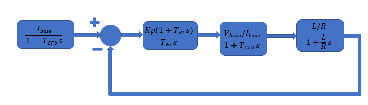
Kp and Ki values for both Id and Iq controllers can be calculated using Modulus optimum theory. As per this theory, the closed-loop system has the following transfer function, which is equivalent to $\begin{array}{l} \frac{I_{f b}}{I_{r e f}} \end{array}$ :

In the above equation and diagram, the terms represent these values:

The equation uses these variables:

$\begin{array}{l} T_{C L D} \end{array}$	Sum of all delays present in the current control loop
$\begin{array}{l} T_{C F b} \end{array}$	Sum of all delays present in feedback path of the current control loop

When no current filter is present and a sensor is used instead of observer, then $\begin{array}{l} T_{C L D} = \frac{T_{s}}{2} + \frac{T_{s}}{2} \end{array}$ . In this case, this is a second order system with these variables:

The variables have these values:

$\begin{array}{l} ζ \end{array}$ (Damping ratio): $\frac{1}{\sqrt{2}}$
$\begin{array}{l} ω_{n} \end{array}$ (Natural frequency): $\begin{array}{l} \frac{1}{\sqrt{2} T_{C L D}} \end{array}$

Speed Control Loop

This image represents the closed-loop transfer function of the speed control loop.

Approximated Block Diagram

The approximated block diagram of speed control loop using transfer functions looks like this:

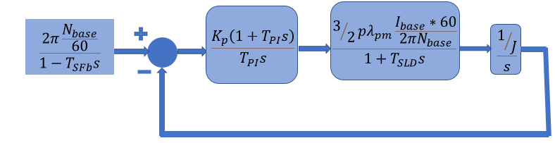
Kp and Ki values for both Id and Iq controllers are calculated using Modulus Optimum theory and we can realize the current control loop as the following first order transfer function:

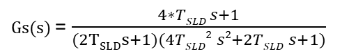
$\begin{array}{l} G c A p p r o x (s) = \frac{1}{s + \frac{1}{T_{C L D}}} \end{array}$

Kp and Ki values for speed controller can be calculated using Symmetric Optimum theory. As per theory, the closed-loop system has following transfer function:

In the above equation and diagram, the terms represent these values:

The equations use these variables:

$\begin{array}{l} T_{S L D} \end{array}$	Time constant for speed control loop delay
$\begin{array}{l} T_{S F b} \end{array}$	Time constant for feedback loop delay during speed control
$\begin{array}{l} T_{C L D} \end{array}$	Sum of all delays present in the current control loop
$\begin{array}{l} T_{C F b} \end{array}$	Sum of all delays present in feedback path of the current control loop
$\begin{array}{l} T_{C L} \end{array}$	Time constant for current control loop delay

You can plot step response for the system along with theoretical approximated transfer function Gs(s). You may see difference in both plots as the gain calculation is done by approximating the system.

Obtain Controller Gains by Providing Basic Electrical and Mechanical Parameters

You can provide values for basic parameters like resistance, inductance, number of pole pairs, FluxPM, sample time of controller, and so on, and run the below code sections that output Kp and Ki values for current control loop and speed control loop.

Run Code for Current Control Loop

Enter the parameter values and click Calculate Gain in this code section to obtain controller gains for current control loop.

%Electrical parameters of motor
R = 0.2; % Stator winding resistance per phase (ohm)
L = 0.002; % d-axis winding inductance (henry)

%Sample time of controller
Ts_curr = 0.00005; % seconds

%Time constant of low pass filter
T_currfilter = 0.0001; % seconds

%Run this section to obtain gains
calculateCLGain;
disp(PIGains);

    Kp: 6.6667
    Ki: 666.6667

Run Code for Speed Control Loop

Enter the parameter values and click Calculate Gain in this code section to obtain controller gains for speed control loop.

%Mechanical parameters of motor
J = 0.001; % Motor inertia (kg-m^2)
p = 4; % Pole-pairs
FluxPM = 1; % Permanent magnet flux linkage (weber)

%Sample time of controller
Ts_spd = 0.001; % seconds

%Time constant of current control loop
T_currloop = 1.5*Ts_curr + T_currfilter; % seconds

%Time constant of low pass filter
T_spdfilter = 0.001; % seconds

%Run this section to obtain gains
calculateSLGain;
disp(PIGains);

    Kp: 0.0383
    Ki: 4.4039

Simulate Model to Obtain Controller Gains for Current Control and Speed Control

Alternatively, you can simulate the ModelControlGainBlock model provided with this example, which contains the FOC Default Controller Gains block. Provide the basic parameters, sample time, and time constant values, and so on as inputs to this block and simulate the model to obtain the controller gains.

 
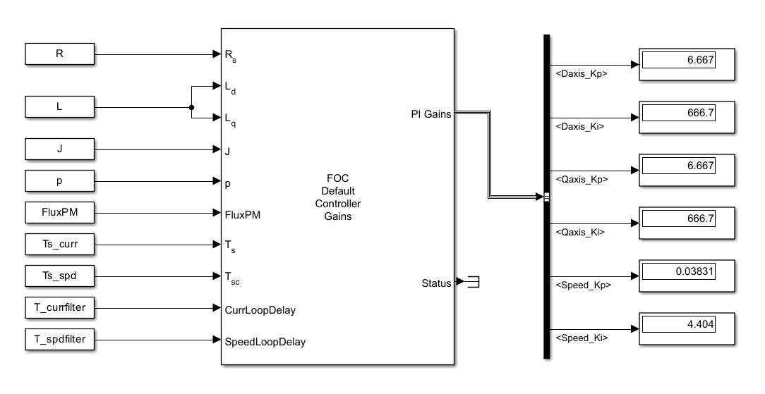
open_system('ModelControlGainBlock');

Obtain Controller Gains for Motor Control Blockset Examples

With Motor Control Blockset™, you can calculate controller gains by applying optimum theories with the capability to consider any number of delays present in the system (for example, delays due to hardware filters and observers (in case of sensorless FOC)). You can use one of the two methods mentioned in this section to perform the approximation of control loops to a lower-order linear time-invariant system. Both the methods use Modulus optimum theory for calculation of current controller gains and Symmetric optimum theory for calculation of speed controller gains.

Define Workspace Variables

Before using the function or block to obtain controller gains, you need to specify values for some Workspace variables. In this example, these values are inputs to the mcb.calcFOCGains function and FOC Default Controller Gains block. These include motor and inverter parameter values, per-unit system base values, PWM switching time period, sample time for the control system, sample time for the speed controller, and filter cutoff frequencies.

%Run this section to define workspace variable
%Select Motor
SelectedMotor = 'Teknic2310P';
pmsm = mcb.getPMSMParameters(SelectedMotor);

%Select Inverter
SelectedInverter = 'BoostXL-DRV8305';
inverter = mcb.getInverterParameters(SelectedInverter);

%Get rated speed for motor and inverter pair
pmsm.N_rated = mcb.getMotorBaseSpeed(pmsm,inverter);

%Choose PWM frequency for controller
PWMFrequency = 20000; % Hz

%Defining sample time for current control loop and speed control loop
Ts = 1/PWMFrequency;
Ts_speed = 10/PWMFrequency;

%Consider board resistance for calculating controller gain
motor = pmsm;
motor.Rs = pmsm.Rs + inverter.R_board;

%Base for SI system
PU_System.V_base = 1; % Volts
PU_System.I_base = 1; % Amperes
PU_System.N_base = 60/(2*pi); % RPM (= 1 rad/sec)
PU_System.T_base = 1; % Nm

% Two low pass filters are connected in series to measure the current signal in the loop 
% only to demonstrate how to use function, if the loop has certain delay component present 
% (either hardware or software). 
% Value of cutoff frequency is chosen randomly.
CutOffFrq1 = 100; % Hz
CutOffFrq2 = 100; % Hz

mcb.calcFOCGains Function

When the motor control application is tailored for a specific motor, you can perform the calculation of gains during the compilation of the controller code. In this scenario, you can use the mcb.calcFOCGains function to determine the controller gains. This example provides details on how to use this function to obtain controller gains for current control loop and speed control loop in FOC of PMSM.

Obtain Gains for Torque or Current Control Loop Using mcb.calcFOCGains

% Command to obtain gain
PI_params = mcb.calcFOCGains(motor,Ts,Ts_speed);

Simulate the model and plot the step response for the system along with theoretical approximated transfer function Gc(s). You may see difference in both plots as the gain calculation is done by approximating the system.

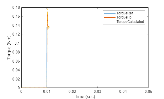
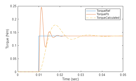
% Run this section to simulate model and plot torque step responses of the modeled torque
% control loop (TorqueFb) and the approximated transfer function (TorqueCalculated)
T = Ts; % Total delay (Here, T = T_CLD from the equation)
plotStepResponse('ModelForTorqueControl','UsingScript','SI','WithoutDelay');

Figure contains an axes object. The axes object with xlabel Time (sec), ylabel Torque (Nm) contains 3 objects of type line. These objects represent TorqueRef, TorqueFb, TorqueCalculated.

Controller Gains Based on Per-Unit System Using mcb.calcFOCGains

In this section, you replace the initial values that were used by the function with per-unit values instead.

%Run this section to define base values for PU system
PU_System.V_base = inverter.V_dc/sqrt(3);
PU_System.I_base = pmsm.I_rated;
PU_System.N_base = pmsm.N_rated;
PU_System.T_base = pmsm.T_rated;

% Use input argument 'Base' to provide base values defined for system 
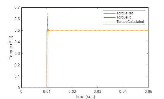
PI_params = mcb.calcFOCGains(pmsm,Ts,Ts_speed,Base=PU_System);

% Run this section to simulate model and plot torque step responses of modeled torque
% control loop (TorqueFb) and the approximated transfer function (TorqueCalculated)
plotStepResponse('ModelForTorqueControl','UsingScript','PU','WithoutDelay');

Figure contains an axes object. The axes object with xlabel Time (sec), ylabel Torque (PU) contains 3 objects of type line. These objects represent TorqueRef, TorqueFb, TorqueCalculated.

Controller Gains Based on SI System Using mcb.calcFOCGains With One Delay Element

In this section, you add a delay element in the feedback path and obtain control gains for current control loop control.

%Run this section to consider delay in the loop
%Select cutoff frequency
CutOffFrq = 100; % Hz
%Create delay component to represent filter
Delay.Gain = 1;
Delay.TimeConstant = 1/(2*pi*CutOffFrq);

%Input argument 'CLFeedbackPathDelay' is used to define a delay element in
%feedback path of the current control loop (CL)
PI_params = mcb.calcFOCGains(pmsm,Ts,Ts_speed,CLFeedbackPathDelay=Delay);

In the below code, T is $\begin{array}{l} T_{C L D} \end{array}$ as represented in the transfer function for Gc(s).

% Run this section to simulate model and plot torque step responses of modeled torque
% control loop (TorqueFb) and the approximated transfer function (TorqueCalculated)
T = Ts + Delay.TimeConstant; % Total delay (Here T is T_CLD)
plotStepResponse('ModelForTorqueControl','UsingScript','SI','WithDelay');

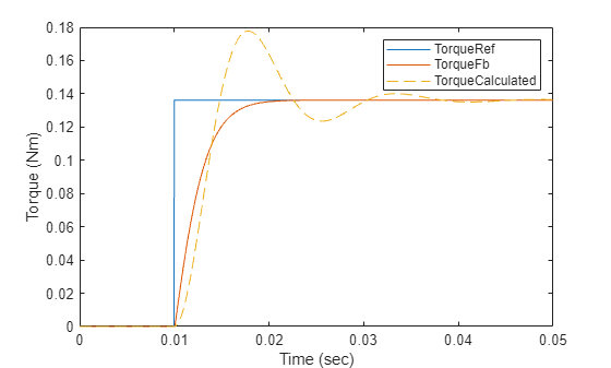
Figure contains an axes object. The axes object with xlabel Time (sec), ylabel Torque (Nm) contains 3 objects of type line. These objects represent TorqueRef, TorqueFb, TorqueCalculated.

Note: The difference in dynamics between the calculated torque and the simulation result is because of the approximation of the transfer function

Controller Gains Based on SI System Using mcb.calcFOCGains With Two Delay Elements

In this section, you add multiple delay elements (for example, hardware low pass filter, software low pass filter, or observer) in the feedback path and obtain control gains for current control loop..

% Run this section to add two delay in series for the loop
% Select cutoff frequency for first filter
CutOffFrq = 500; % Hz
% Create delay component to represent filter
Delay1.Gain = 1;
Delay1.TimeConstant = 1/(2*pi*CutOffFrq);
% Select cutoff frequency for second filter
CutOffFrq = 500; % Hz
% Create delay component to represent filter
Delay2.Gain = 1;
Delay2.TimeConstant = 1/(2*pi*CutOffFrq);
TotalDelay.Gain = [Delay1.Gain Delay2.Gain];
TotalDelay.TimeConstant = [Delay1.TimeConstant Delay2.TimeConstant];

% Input argument 'CLFeedbackPathDelay' to define all delay elements in
% feedback path of the current control loop (CL)
PI_params = mcb.calcFOCGains(pmsm,Ts,Ts_speed,CLFeedbackPathDelay=TotalDelay);

In the below code, T is $\begin{array}{l} T_{C L D} \end{array}$ as represented in the transfer function for Gc(s).

% Run this section to simulate model and plot torque step responses of modeled torque
% control loop (TorqueFb) and the approximated transfer function (TorqueCalculated)
T = Ts + Delay1.TimeConstant + Delay2.TimeConstant; % Total delay (Here T is T_CLD)
plotStepResponse('ModelForTorqueControl','UsingScript','SI','WithTwoDelays');

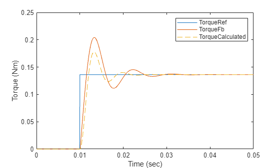
Figure contains an axes object. The axes object with xlabel Time (sec), ylabel Torque (Nm) contains 3 objects of type line. These objects represent TorqueRef, TorqueFb, TorqueCalculated.

Note: The difference in dynamics between the calculated torque and the simulation result is because of the approximation of the transfer function.

FOC Default Controller Gains Block

When motor control application needs to operate with different motor setups without recompiling the code each time, you need to integrate the calculation of gains into the controller code. In this scenario, you can use the FOC Default Controller Gains block to determine the controller gains during runtime. The Simulink models in this example use this block to obtain controller gains for current control loop and speed control loop in FOC of PMSM.

Obtain Controller Gains for Torque or Current Control Using FOC Default Controller Gains Block

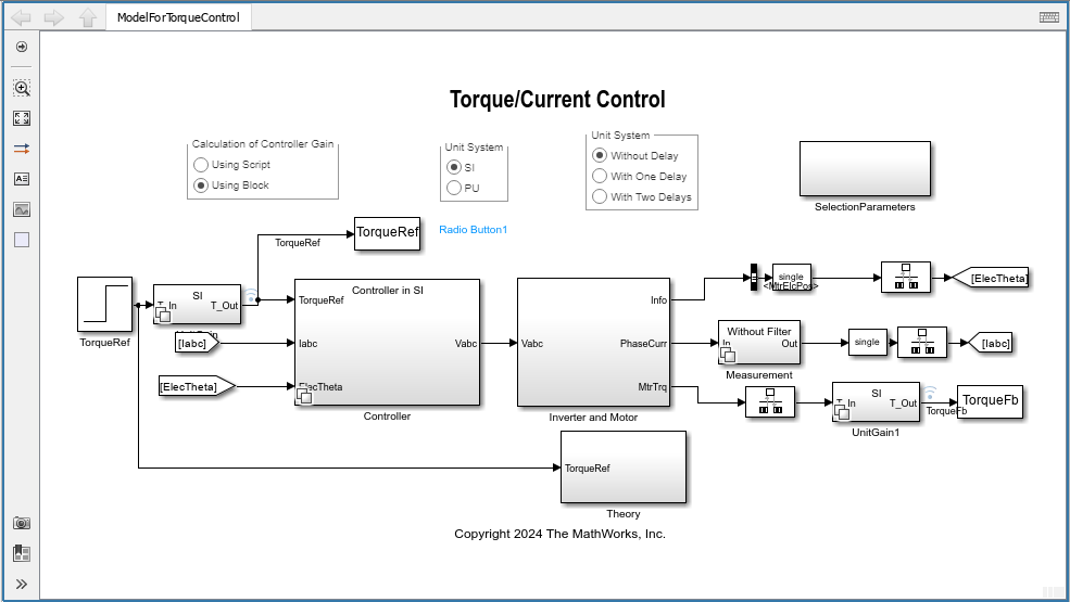
%Run this section to open the model
openModel('ModelForTorqueControl','UsingBlock','SI','WithoutDelay');

The Controller/Controller Gain subsystem in the model contains the FOC Default Controller Gains Block. You can simulate the model to obtain controller gains that is the input to the Field-Oriented Current Controller block in the Controller subsystem.

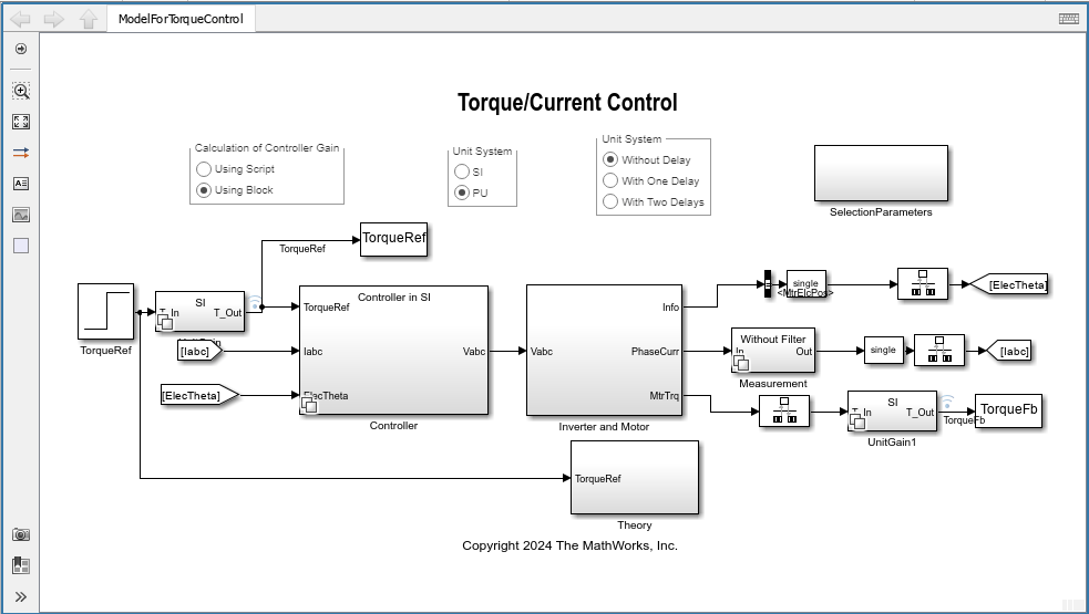
Controller Gains Based on Per-Unit System Using FOC Default Controller Gains Block

In this section, you replace the initial values that were used by the block with per-unit values instead.

%Run this section to open the model
openModel('ModelForTorqueControl','UsingBlock','PU','WithoutDelay');

Simulate the model to obtain controller gains that is the input to the Field-Oriented Current Controller block in the Controller subsystem.

Controller Gains Based on SI System FOC Default Controller Gains Block With One Delay Element

%Run this section to open the model
openModel('ModelForTorqueControl','UsingBlock','SI','WithDelay');

Simulate the model to obtain controller gains that is the input to the Field-Oriented Current Controller block in the Controller subsystem.

Controller Gains Based on SI System FOC Default Controller Gains Block With Two Delay Elements

%Run this section to open the model
openModel('ModelForTorqueControl','UsingBlock','SI','WithTwoDelays');

Obtain Gains for Torque Control with Slow Response

When there is an unknown delay component present in the system, you can use a slow-down factor for calculating controller gains.

%Run this section to add slow down factor in torque control loop
%Select slow down factor
Factor = 0.25;
PI_params = mcb.calcFOCGains(pmsm,Ts,Ts_speed,DCurrLoopFactor=Factor,QCurrLoopFactor=Factor);

%Run this section to simulate model and plot torque step responses of modeled torque
%control loop (TorqueFb) and the approximated transfer function (TorqueCalculated)
T = Ts + 1/(2*pi*CutOffFrq1);
plotStepResponse('ModelForTorqueControl','UsingScript','SI','WithDelay');

Figure contains an axes object. The axes object with xlabel Time (sec), ylabel Torque (Nm) contains 3 objects of type line. These objects represent TorqueRef, TorqueFb, TorqueCalculated.

Note: The difference in dynamics between the calculated torque and the simulation result is because of the approximation of the transfer function.

Obtain Gains for Speed Control Loop Using mcb.calcFOCGains

%Run this section to obtain gain for speed control loop
%Base for SI system
PU_System.V_base = 1; % V
PU_System.I_base = 1; % A
PU_System.N_base = 60/(2*pi); % RPM (= 1 rad/sec)
%Define coefficient for IIR filter present for measured speed
SpdCoeff = 0.05;
PI_params = mcb.calcFOCGains(motor,Ts,Ts_speed,SpdLPFltCoeff=SpdCoeff);

%Run this section to simulate model and plot torque step responses of the modeled
%speed control loop (SpeedFb) and the approximated transfer function (SpeedCalculated)
T = 1.5*Ts + Ts_speed + Ts*(1-SpdCoeff)/SpdCoeff; % Here T = T_SLD
plotStepResponse('ModelForSpeedControl','UsingScript','SI','WithoutDelay');

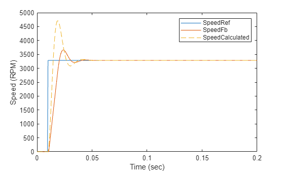
Figure contains an axes object. The axes object with xlabel Time (sec), ylabel Speed (RPM) contains 3 objects of type line. These objects represent SpeedRef, SpeedFb, SpeedCalculated.

Note: The difference in dynamics between the calculated speed and the simulation result is because of the approximation of the transfer function.

Obtain Gains and Plot Response for Speed Control Based on Per-Unit System Using mcb.calcFOCGains

In this section, you replace the initial values that were used by the function with per-unit values instead.

%Run this section to define base values for PU system
PU_System.V_base = inverter.V_dc/sqrt(3);
PU_System.I_base = pmsm.I_rated;
PU_System.N_base = pmsm.N_rated;
PU_System.T_base = pmsm.T_rated;

%Use input argument 'Base' to provide base values defined for system 
PI_params = mcb.calcFOCGains(pmsm,Ts,Ts_speed,SpdLPFltCoeff=SpdCoeff,Base=PU_System);

%Run this section to simulate model and plot torque step responses of modeled
%speed control loop (SpeedFb) and the approximated transfer function (SpeedCalculated)
T = 1.5*Ts + Ts_speed + Ts*(1-SpdCoeff)/SpdCoeff;
plotStepResponse('ModelForSpeedControl','UsingScript','PU','WithoutDelay')

Figure contains an axes object. The axes object with xlabel Time (sec), ylabel Speed (PU) contains 3 objects of type line. These objects represent SpeedRef, SpeedFb, SpeedCalculated.

Note: There is a difference in dynamics between theory and simulation due to the approximation of the transfer function.

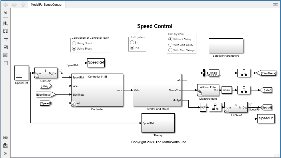
Obtain Gains for Speed Control Loop Using FOC Default Controller Gains Block

%Run this section to open the model
openModel('ModelForSpeedControl','UsingBlock','SI','WithoutDelay');

The Controller/Controller Gain subsystem in the model contains the FOC Default Controller Gains Block. Simulate the model to obtain controller gains that is the input to the Field-Oriented Current Controller block in the Controller subsystem.

Obtain Gains Based on Per-Unit System for Speed Control Using FOC Default Controller Gains Block

In this section, you replace the initial values that were used by the block with per-unit values instead.

%Run this section to open the model
openModel('ModelForSpeedControl','UsingBlock','PU','WithoutDelay');

Simulate the model to obtain controller gains that is the input to the Field-Oriented Current Controller block in the Controller subsystem.

Obtain Gain for Speed Control with Slow Response

When there is an unknown delay component present in the system, you can use a slow-down factor for calculating controller gains.

%Run this section to add slow down factor for speed control loop
% Select slow down factor
Factor = 0.5;
PI_params = mcb.calcFOCGains(pmsm,Ts,Ts_speed,SpdLPFltCoeff=0.1,SpdLoopFactor=Factor,Base=PU_System);

%Run this section to simulate model and plot torque step responses of modeled
%speed control loop (SpeedFb) and the approximated transfer function (SpeedCalculated)
T = 1.5*Ts + Ts_speed + Ts*(1-SpdCoeff)/SpdCoeff;
plotStepResponse('ModelForSpeedControl','UsingScript','PU','WithoutDelay');

Figure contains an axes object. The axes object with xlabel Time (sec), ylabel Speed (PU) contains 3 objects of type line. These objects represent SpeedRef, SpeedFb, SpeedCalculated.

Note: The difference in dynamics between the calculated speed and the simulation result is because of the approximation of the transfer function.

Advanced Capabilities of mcb.calcFOCGains for OLTF and CLTF

The mcb.calcFOCGains function also outputs open-loop transfer function (OLTF) and close-loop transfer function (CLTF) for each of the three loops (D-axis current, Q-axis current, and Speed).

Note: You require Control System Toolbox™ license to compute the transfer function using mcb.calcFOCGains function.

For example:

[PI_params,OLTF,CLTF] = mcb.calcFOCGains(motor,Ts,Ts_speed);
% Open loop transfer function for D-axis current control loop
DCurrOpenLoopTF = tf(OLTF.DCurrLoop.Numerator,OLTF.DCurrLoop.Denominator)

DCurrOpenLoopTF =
 
               2.745
  -------------------------------
  2.745e-08 s^2 + 0.0005989 s + 1
 
Continuous-time transfer function.
Model Properties

% Open loop transfer function for Q-axis current control loop
QCurrOpenLoopTF = tf(OLTF.QCurrLoop.Numerator,OLTF.QCurrLoop.Denominator)

QCurrOpenLoopTF =
 
               2.745
  -------------------------------
  2.745e-08 s^2 + 0.0005989 s + 1
 
Continuous-time transfer function.
Model Properties

% Open loop transfer function for speed control loop
SpeedOpenLoopTF = tf(OLTF.SpdLoop.Numerator,OLTF.SpdLoop.Denominator)

SpeedOpenLoopTF =
 
        5434
  ----------------
  0.000575 s^2 + s
 
Continuous-time transfer function.
Model Properties

% Closed loop transfer function for D-axis current control loop
DCurrCloseLoopTF = tf(CLTF.DCurrLoop.Numerator,CLTF.DCurrLoop.Denominator)

DCurrCloseLoopTF =
 
          2e08
  --------------------
  s^2 + 20000 s + 2e08
 
Continuous-time transfer function.
Model Properties

% Closed loop transfer function for Q-axis current control loop
QCurrCloseLoopTF = tf(CLTF.QCurrLoop.Numerator,CLTF.QCurrLoop.Denominator)

QCurrCloseLoopTF =
 
          2e08
  --------------------
  s^2 + 20000 s + 2e08
 
Continuous-time transfer function.
Model Properties

% Closed loop transfer function for speed control loop
SpeedCloseLoopTF = tf(CLTF.SpdLoop.Numerator,CLTF.SpdLoop.Denominator)

SpeedCloseLoopTF =
 
                  0.0023 s + 1
  --------------------------------------------
  1.521e-09 s^3 + 2.645e-06 s^2 + 0.0023 s + 1
 
Continuous-time transfer function.
Model Properties

For more information about performing control analysis for the above transfer function object, refer to Get Started with Control System Toolbox.