Logging Accelerometer Data
This example shows how to manipulate and visualize data coming from a smartphone or tablet accelerometer.
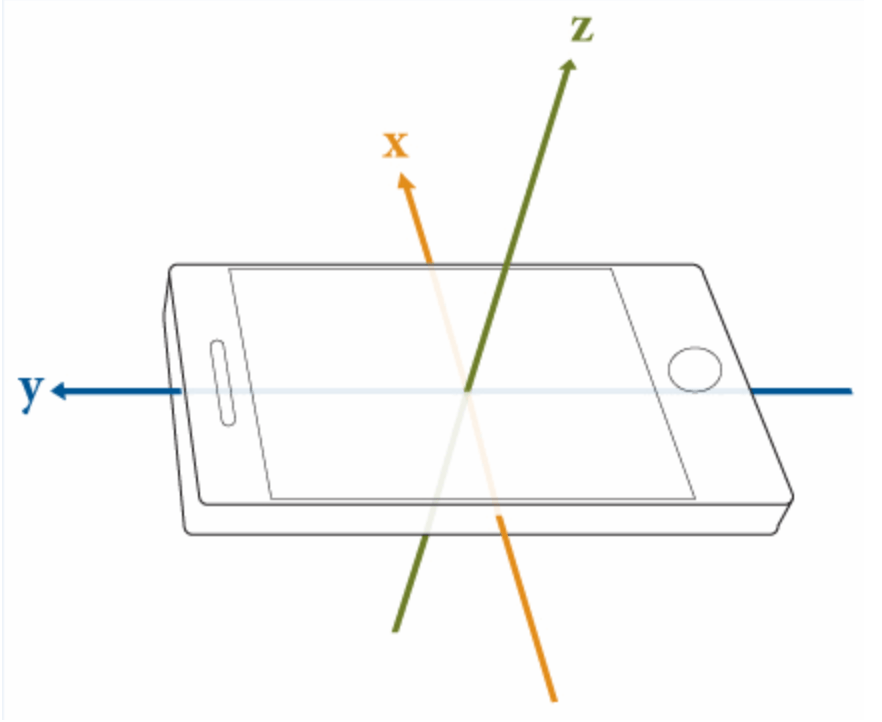
The accelerometer is a sensor that measures the rate of change of velocity, the acceleration. It uses a 3-dimensional cartesian coordinate system and returns acceleration values for each of the axes illustrated in the figure below.
You can easily capture the accelerometer data in MATLAB Mobile using the Sensors menu.

To log accelerometer data, use the following steps:
Select Stream to Log.
Adjust the sample rate (default is 10 Hz).
Turn on the Acceleration switch.
Tap START.
After collecting the data:
Tap STOP.
Enter the file name to be saved (default name is provided).
If you have the Auto Upload option on, the file will be uploaded to your MATLAB Drive as a
.matfile to your configured Upload Folder (default isMATLAB Drive/MobileSensorData).
This example uses a pre-recorded session with the following activities:
Standing
Walking
Jogging
Sprinting
The data was collected with the smartphone attached to the chest of the athlete in portrait orientation with the screen facing forward.
To visualize the data, first load the .mat file of captured sensor data.
load fieldActivities.matRead the data into variables x, y, z and the timestamps into timestamp.
x = Acceleration.X;
y = Acceleration.Y;
z = Acceleration.Z;
timestamp = Acceleration.Timestamp;
With the acceleration values in the loaded variables, calculate the magnitude of the combined 3-axes vector.
combinedAccel = sqrt(x.^2+y.^2+z.^2);
Initialize a vector t with zeros (recommended for performance).
t = zeros(size(timestamp));
Convert the absolute time into relative values setting the start as reference.
for n = 1 : length(timestamp)
  t(n) = seconds(timestamp(n) - timestamp(1));
end
Finally, use the plot command to display the results.
plot(t, combinedAccel)
xlabel('Time (s)')
ylabel('Acceleration (m/s^2)')
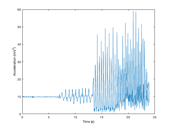
You can easily identify the four different activities in the graph. It starts with the standing position, where the acceleration is nearly constant at 9.8 m/s^2 (gravity), then both amplitude and frequency increase as the activity progresses to walking, jogging, and sprinting.
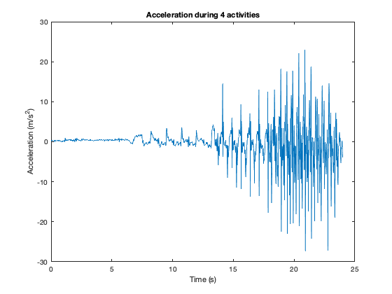
If you want to see individual results for each axis, use the live control below.
Select the axis to see acceleration values in that direction.
plot (t,x)
title('Acceleration during 4 activities')
xlabel('Time (s)')
ylabel('Acceleration (m/s^2)')